[Grasshopper] How to use Field Line to create curves reflecting magnetic fields

This article explains how to use Field Line to create curves reflecting magnetic fields.

On the Grasshopper, it is represented by either of the two above.

Create a curve reflecting magnetic fields

Using Field Line allows you to create curves that reflect magnetic fields.

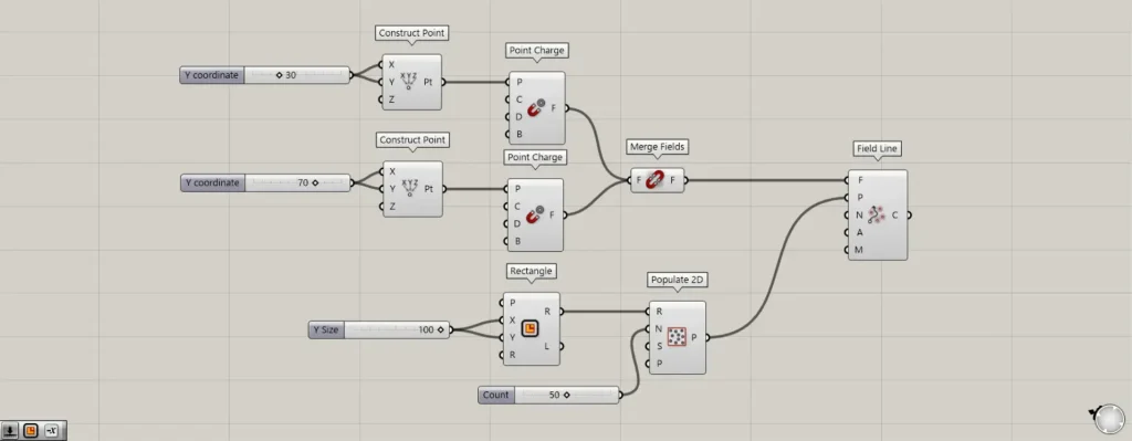
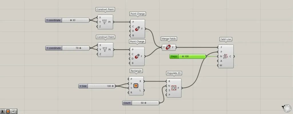
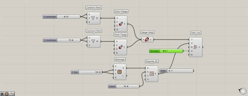
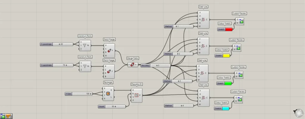
Components used: ①Construct Point ②Point Charge ③Merge Fields ④Rectangle ⑤Populate 2D ⑥Field Line

As an example, let’s create a curve reflecting two magnetic fields.

First, we will create a magnetic field.

Prepare two Construct Point.

Enter 30 into the first Construct Point(X and Y).

Enter 70 into the second Construct Point(X and Y).

Then, points are created at the coordinates 30,30,0 and 70,70,0, respectively.

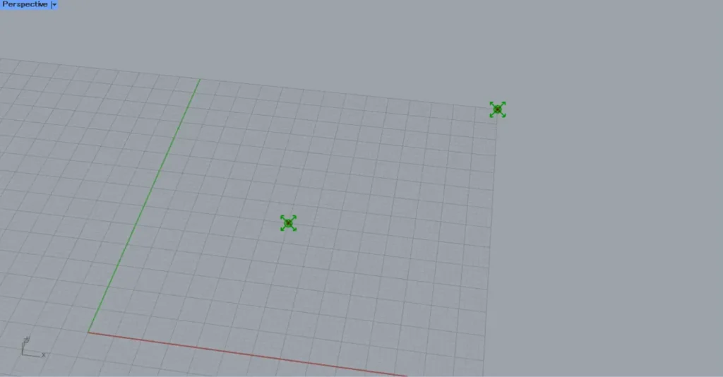
Connect the two Construct Points to the Point Charge(P), respectively.

Then, a magnetic field is created at the specified point.

Then connect two Point Charges to the Merge Fields.

This combines the two magnetic fields into one.

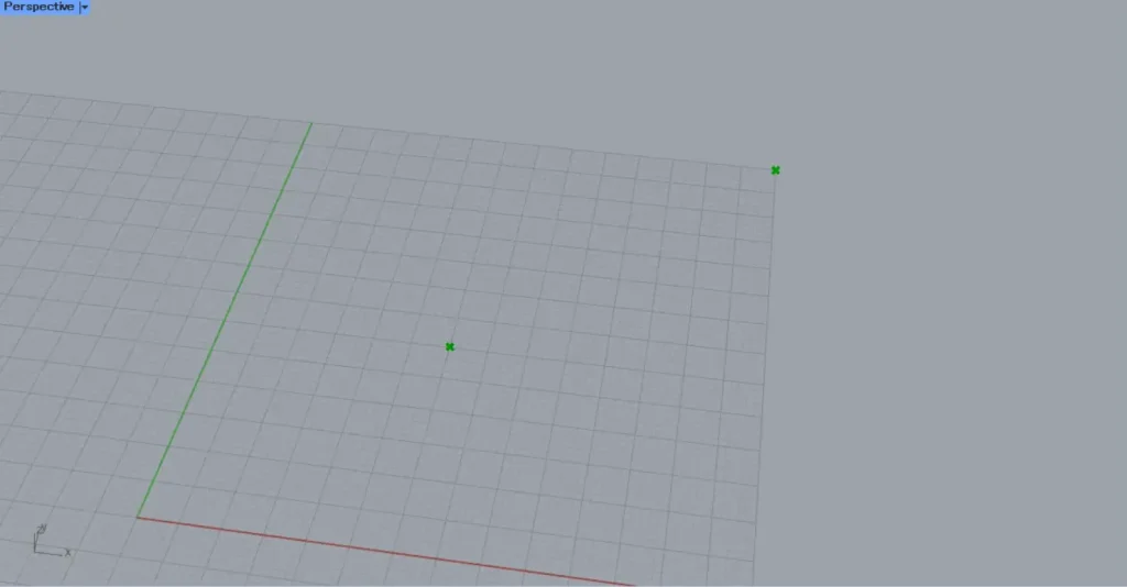
Next, we will create the point data that will serve as the starting point for the curve we are creating.

This time, we will create points randomly within a rectangle.

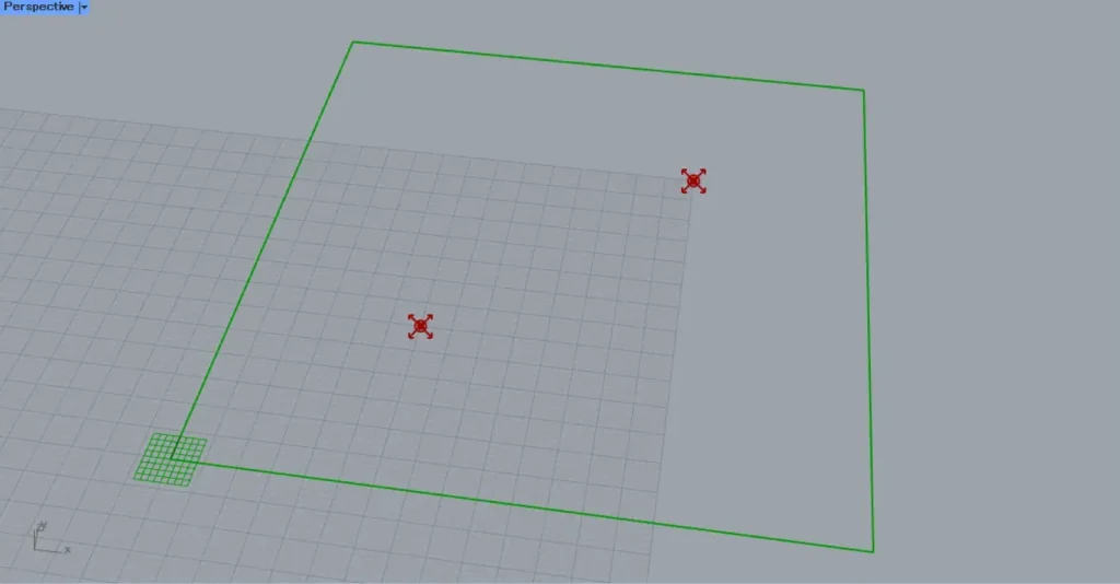
First, enter 100 into the Rectangle(X and Y) to create a 100×100 rectangle.

Next, connect the Rectangle(R) to the Populate 2D(R).

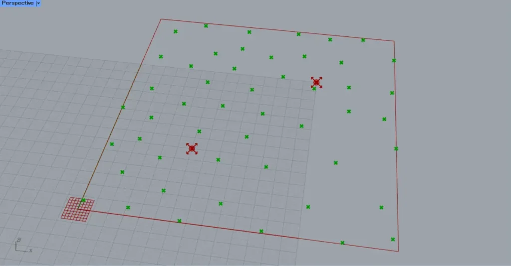
Then, enter the number of points to create into the Populate 2D(N).

This time, since 50 was entered, 50 points were created.

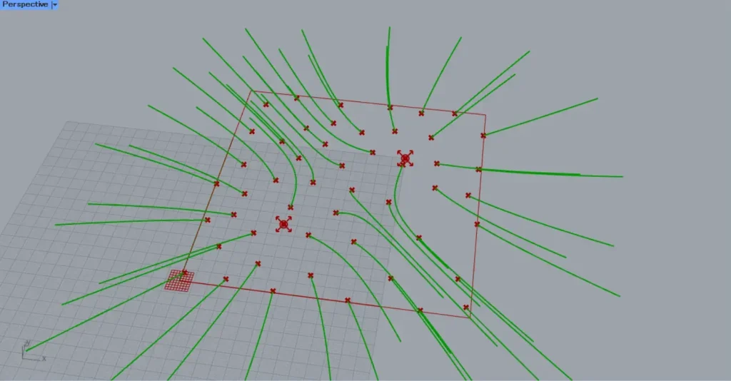
Then, connect the Merge Fields to the Field Line(F).

Additionally, connect Populate 2D to the Field Line(P).

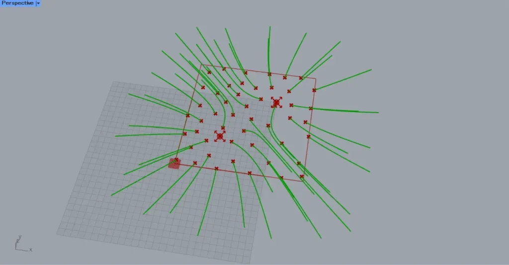
Then, curves reflecting the magnetic field was created starting from the specified points.

In this way, by using the Field Line, you can create curves influenced by the magnetic field.

You can change the curve length by entering a value in the N terminal of Field Line.

The entered value represents the number of Steps, not the curve’s length. To visualize this, think of how the curve changes over time.

First, let’s try entering 100 into the N terminal.

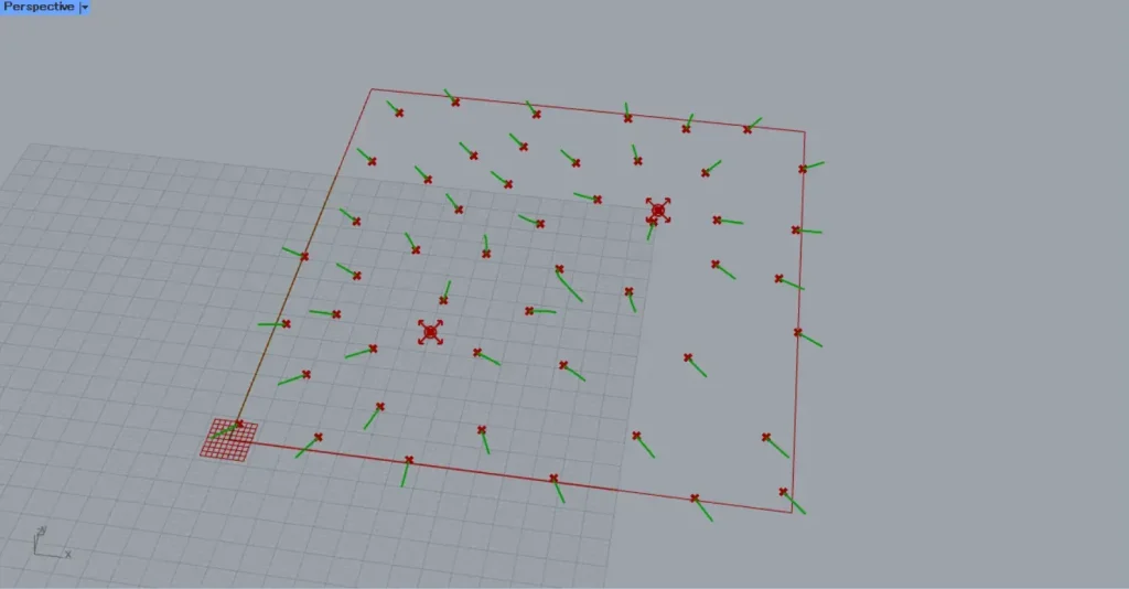
This is what happens when you input 100 into the N terminal.

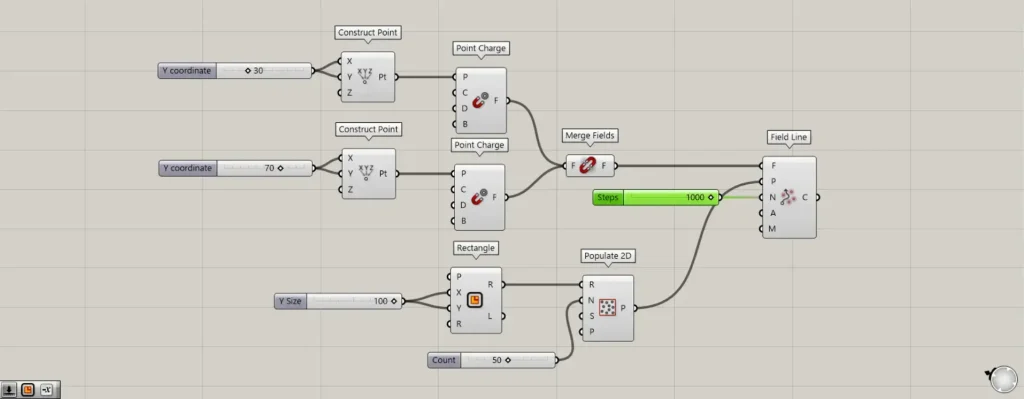
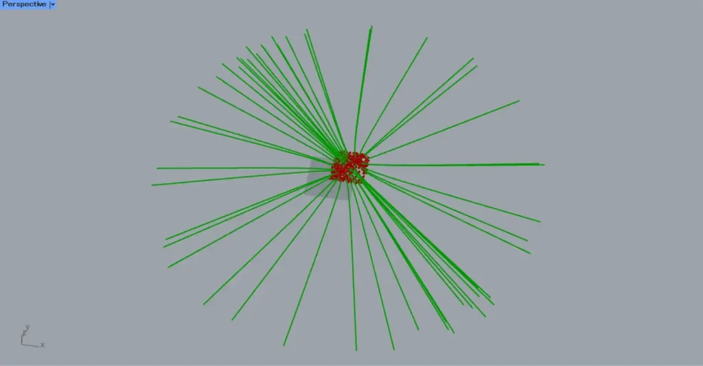
Next, let’s input 1000 into the N terminal.

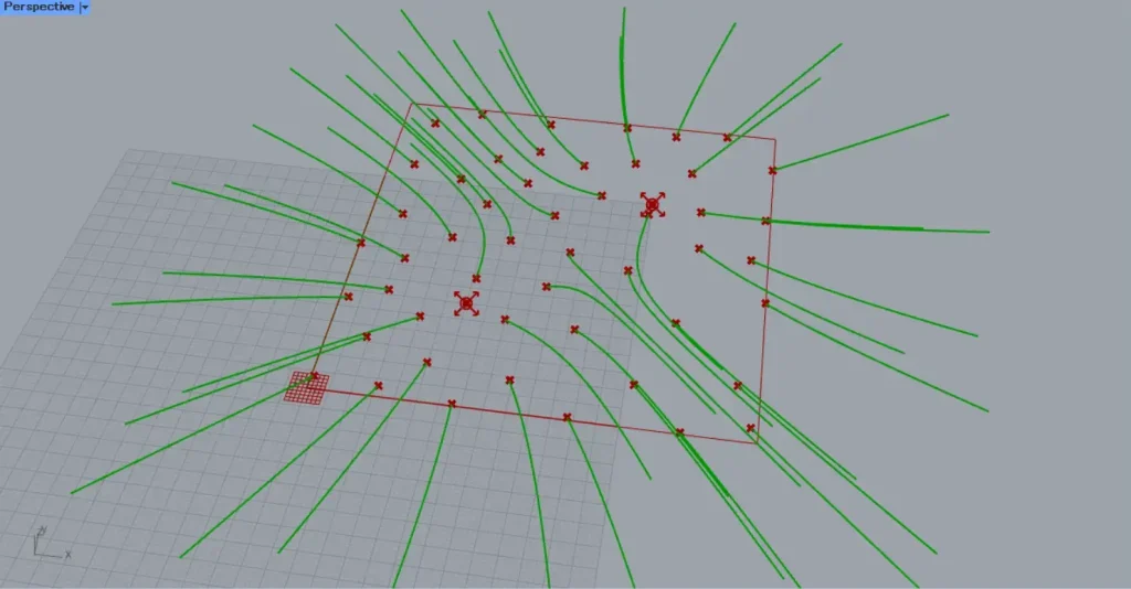
Then, the length of the curve changed like this.

You can also change the length by entering a decimal value into terminal A.

First, let’s try entering 0.1.

This shows what happens when a value of 0.1 is entered into Terminal A.

Next, let’s input the value 1.0 into terminal A.

This is what happens when you input the value 1.0 into Terminal A.

In this way, even decimal points can alter the length of a curve.

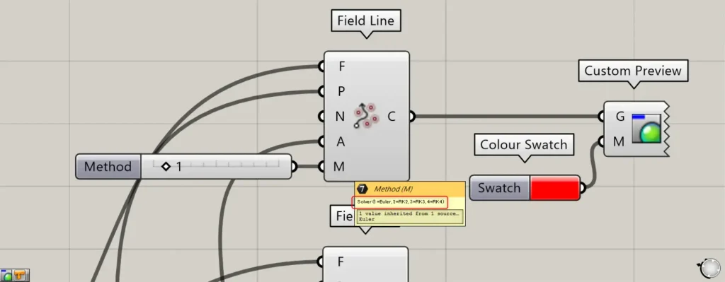
For the M terminal, you can select the curve type by entering values from 1 to 4.

If the value is 1, it becomes Euler; if 2, RK2; if 3, RK3; if 4, RK4.

Additional Components: ①Custom Preview ②Color Swatch

Prepare four Field Lines with values 1 through 4 entered into the M terminals, and connect them to the Custom Preview(G).

Then, specify each color in Colour Swatch, connect it to the Custom Preview(M), and change the colors to observe the four curves.

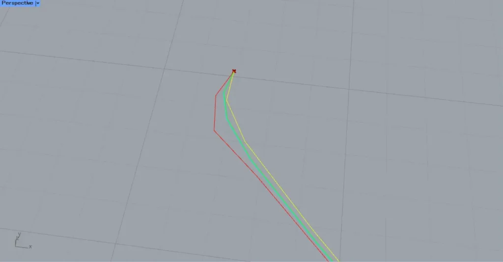
Then, you can see that the curve types have changed as shown here.

List of Grasshopper articles using Field Line component↓

Field Line

FieldLineコンポーネントを使用しているグラスホッパー記事一覧です。ListofGrasshopperarticlesusingFieldLinecomponent↓

iarchway.com