[Grasshopper] How to use Galapagos for optimization [Data download available]

This article explains how to use Galapagos for optimization.

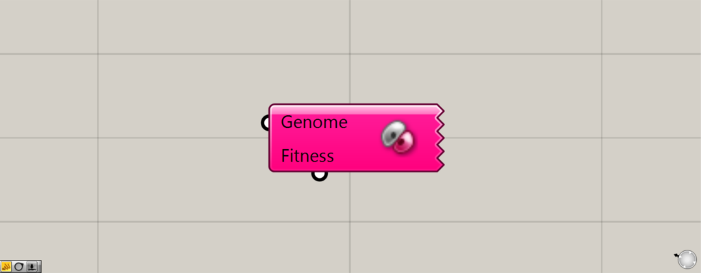
On the Grasshopper, the component is shown in the image above.

The Grasshopper data used in this article is available for download.

Click here to download the Grasshopper data used in this article.

Please refer to the Terms of Use regarding the use of downloadable data.

Video of Galapagos in use

What Galapagos can do

With Galapagos, you can optimize a numerical value to a maximum or minimum from the variables you enter.

It is also possible to optimize to an arbitrary number depending on your ingenuity and settings.

Two types of optimization methods

Galapagos offers two types of optimization methods.

Evolutionary Solver (Genetic Algorithm)

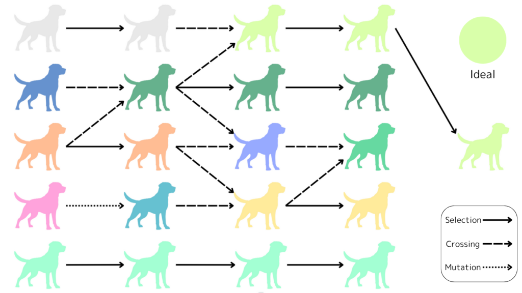
The first method is the Evolutionary Solver (genetic algorithm), which is the default optimization method in Galapagos.

This method is an optimization similar to the process of biological evolution.

From among randomly generated individuals, an individual that is close to the ideal is selected, crossed (two individuals are crossed), and naturally mutated.

By repeating this process for multiple generations, we generate generations that are closer to the ideal, and finally select the most ideal individual from the last generation.

Simulated Annealing Slover

The second method is Simulated Annealing Slover.

This method, named after metallurgical annealing, involves a process in which the metal is heated to a high temperature and then gradually lowered.

The idea that the higher the temperature, the greater the movement of the molecules, and the lower the temperature, the slower the movement of the molecules is used for optimization.

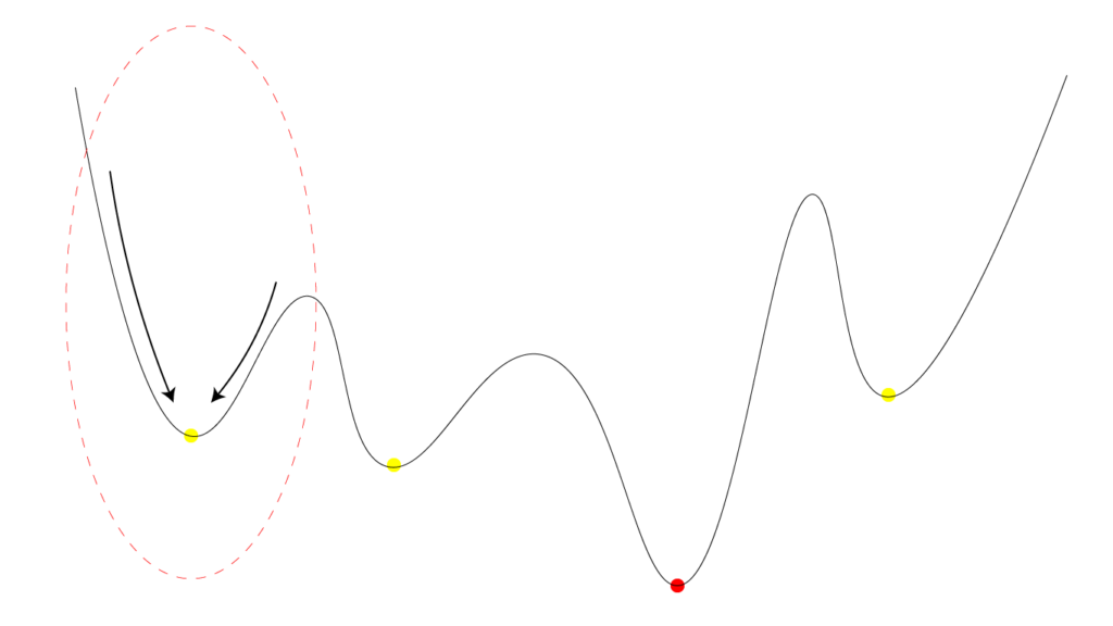
Some optimization methods may reach a locally optimal solution.

In the image above, the red dot is the most ideal result, but if only the left-most range is used, the optimization may be performed within some of the yellow range.

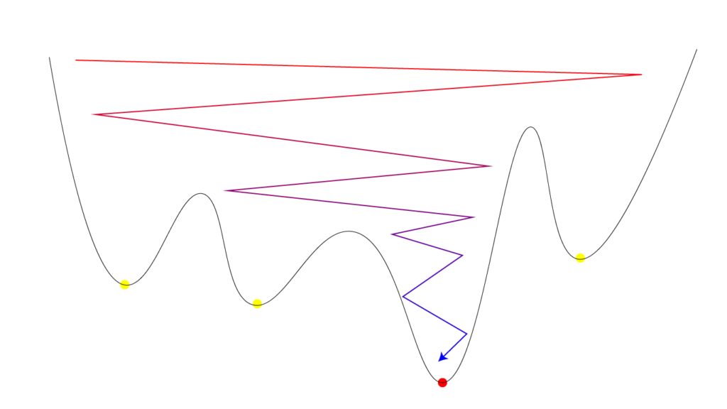
By using Simulated Annealing Slover (annealing method), the entire area is simulated for higher temperatures.

Then, the temperature is gradually lowered and optimization can be done from the range with the globally ideal optimal solution.

How to connect the Fitness and Genome terminals

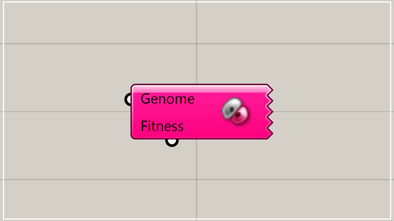
Galapagos has two terminals, Fitness and Genome.

Fitness

Connect the Fitness terminal to the value you want to optimize.

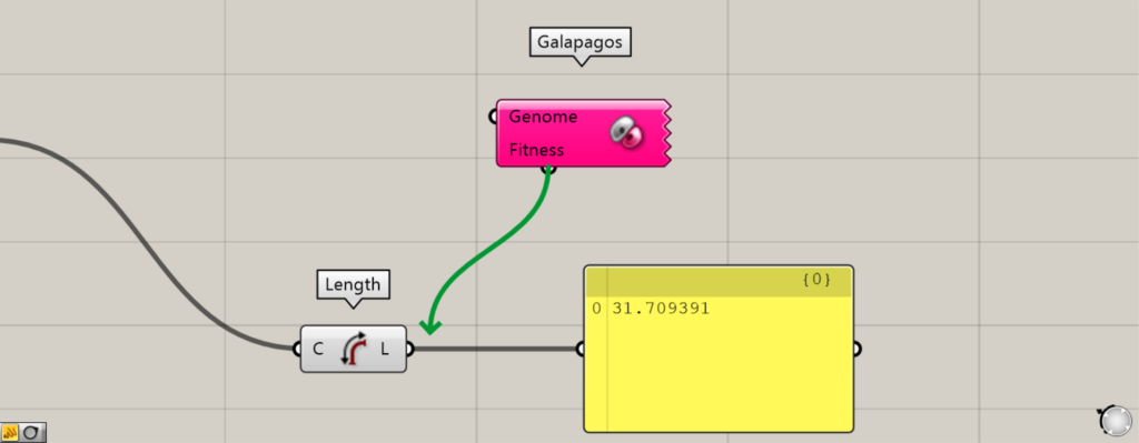
The usual way is to connect the terminals from left to right, but in the case of Galapagos, the terminals are connected from the opposite direction.

Drag the Fitness terminal to the right of the component whose value you want to optimize.

A green arrow will appear.

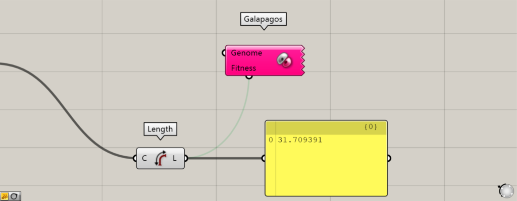
The Fitness terminal is now connected.

Genome

Connect the Genome terminal to the variable value that changes the value you want to optimize.

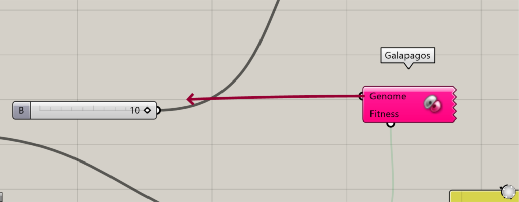
The Genome terminal is also connected from right to left.

Drag the Genome terminal closer to the variable whose value you want to optimize.

A red arrow will even appear.

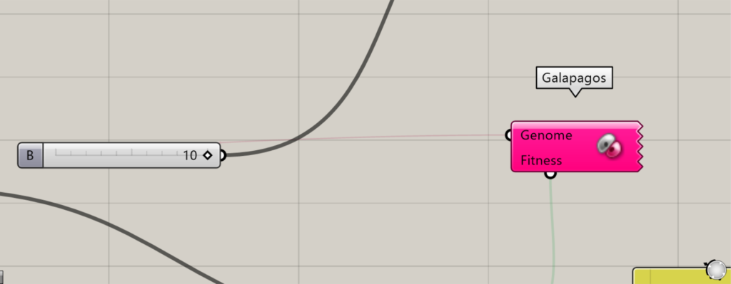
The Genome terminal is now connected.

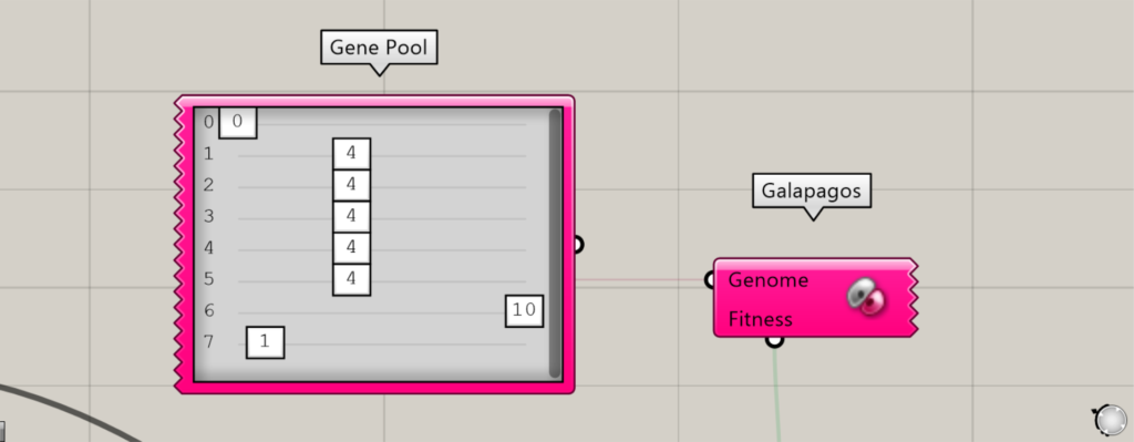
Galapagos variables are often connected to genome terminals using Gene Pools.

By using Gene Pool, multiple variables can be managed in a single component.

In this example, we will also use the Gene Pool.

Basic Optimization Procedure

Let’s take a look at the basic optimization procedure without detailed settings.

First, double-click Galapagos.

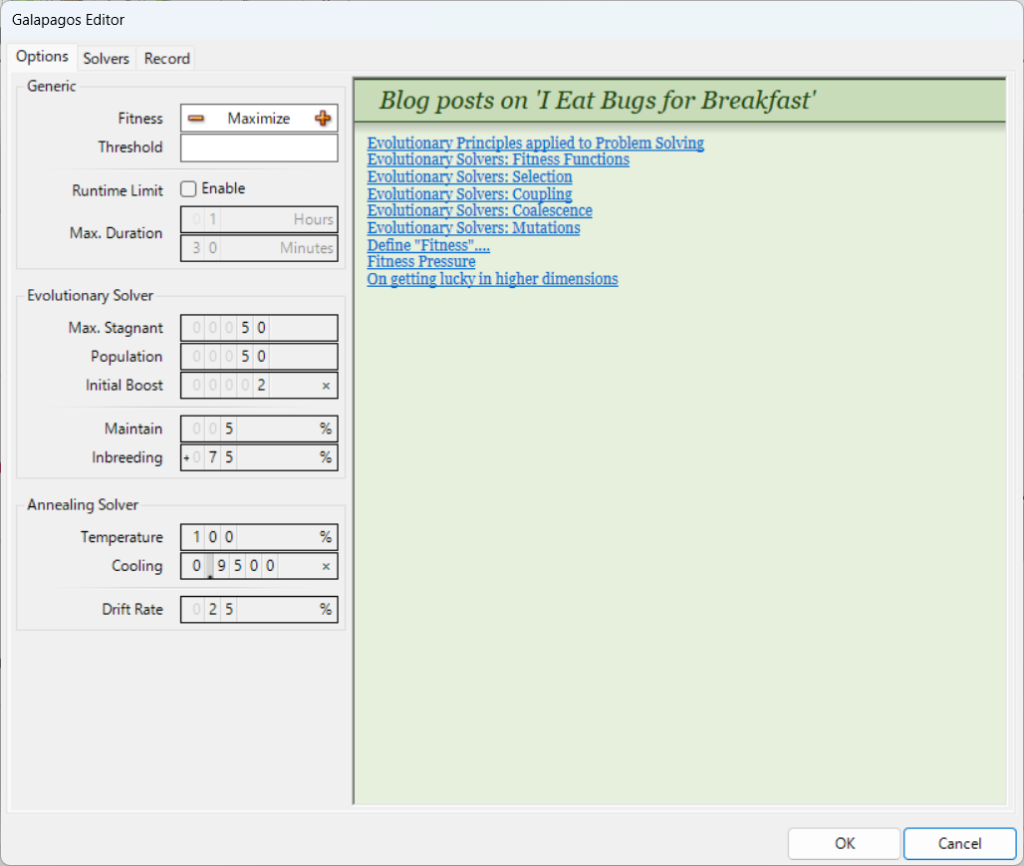
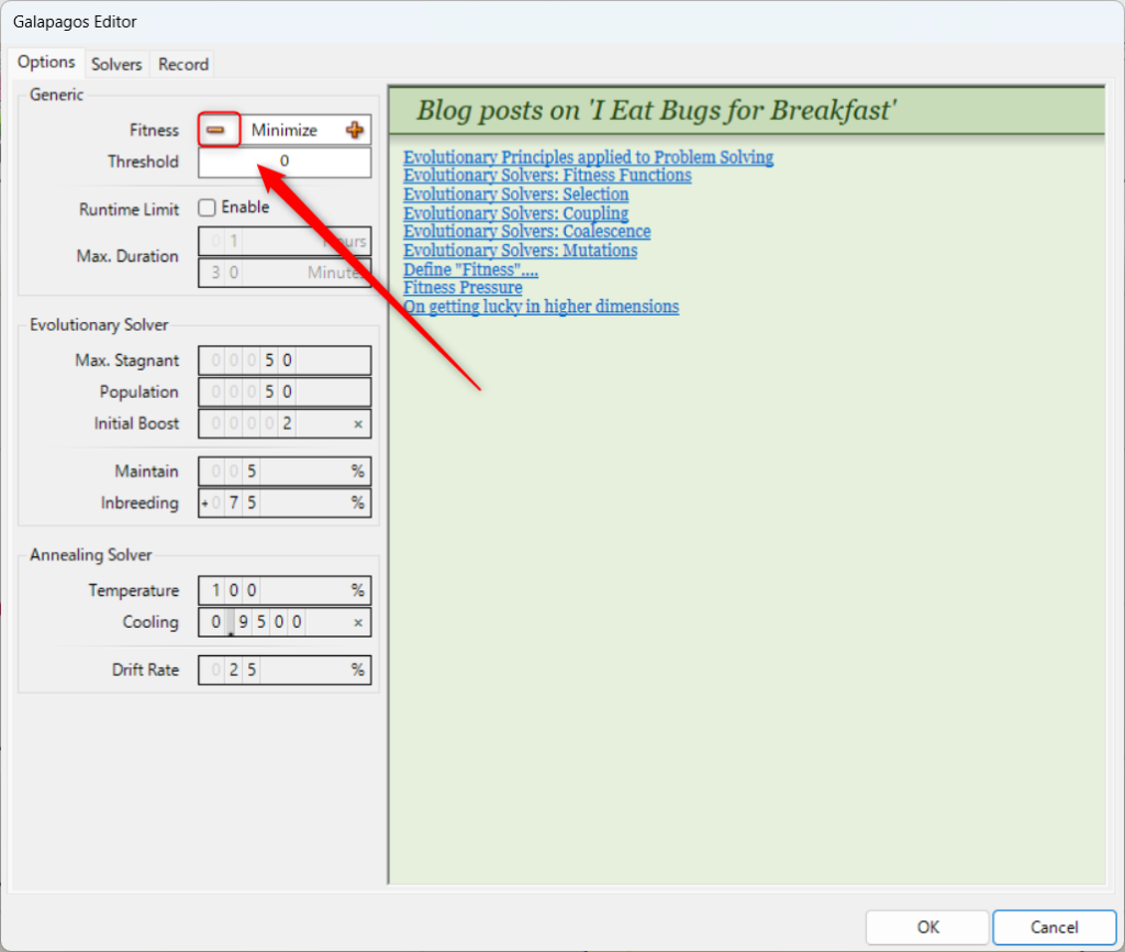
Then, the Galapagos settings screen will appear like this.

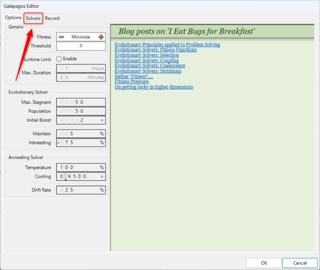
Then, choose whether you want to optimize the values to the maximum or the minimum.

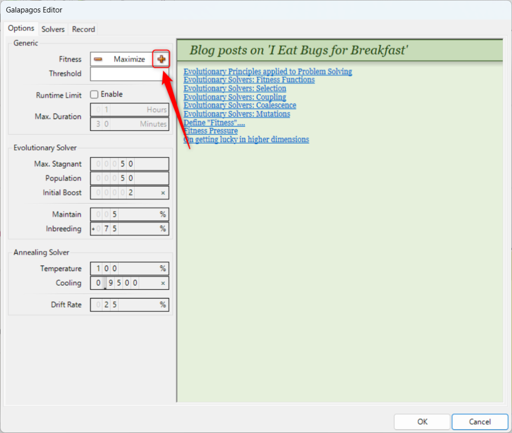
To maximize the values, select the + icon.

The Fitness will then be set to Maximize.

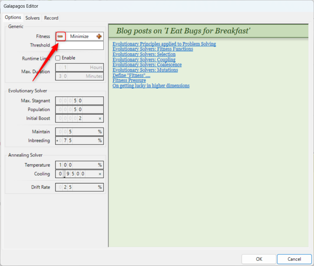
To minimize the value, select the – icon.

The Fitness will then be set to Minimize, which is the setting for minimizing.

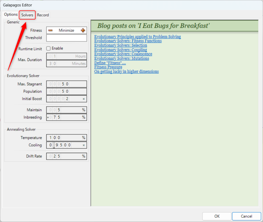
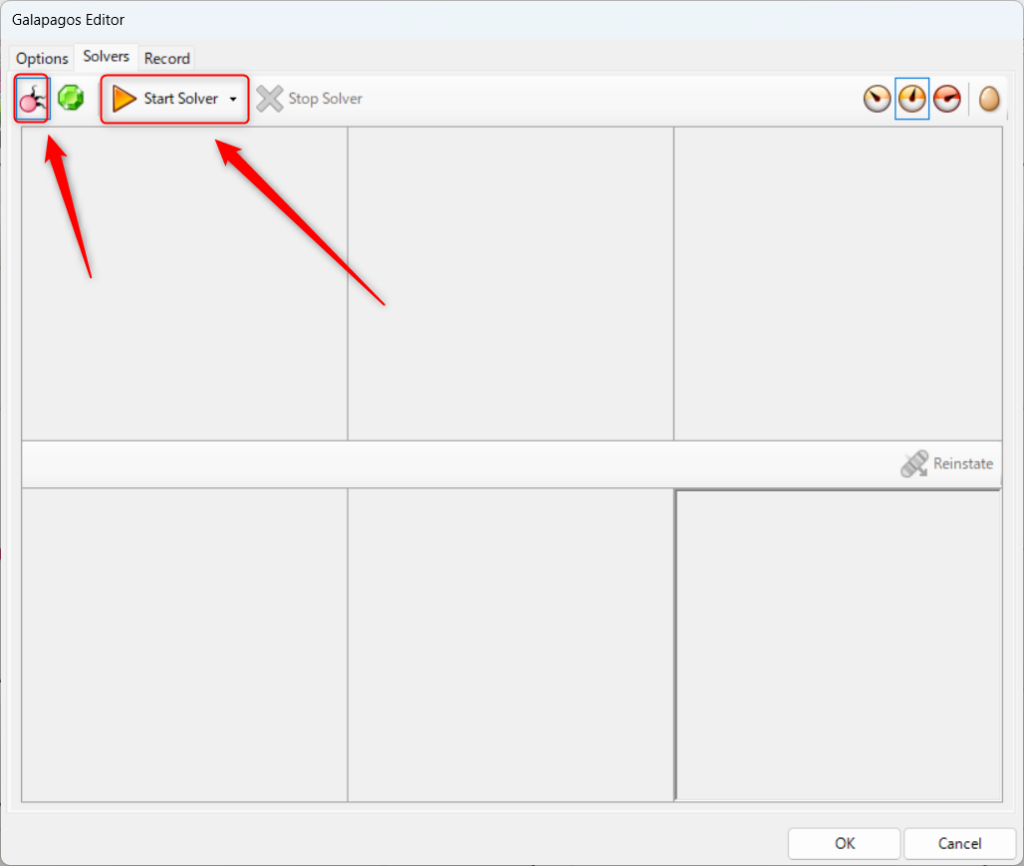
After setting the maximum or minimum value, select the Solvers tab.

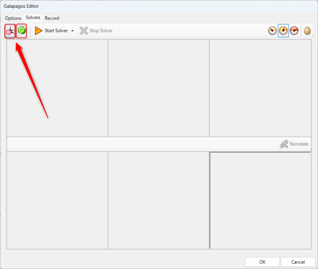
Then select the optimization method.

The icon on the left is the Evolutionary Solver (genetic algorithm) optimization method.

The icon on the right is the Simulated Annealing Slover optimization method.

In this case, we will use the Evolutionary Solver (Genetic Algorithm) on the left.

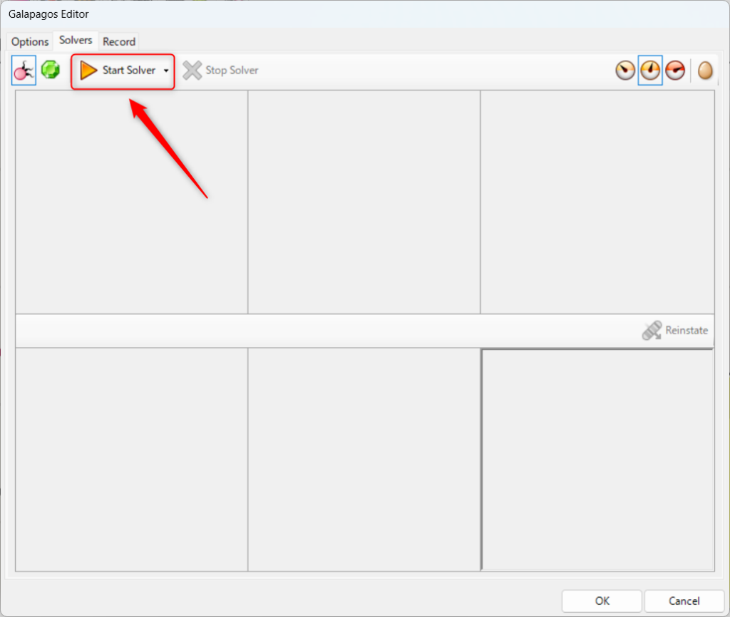
After selecting the optimization method, click Start Solver.

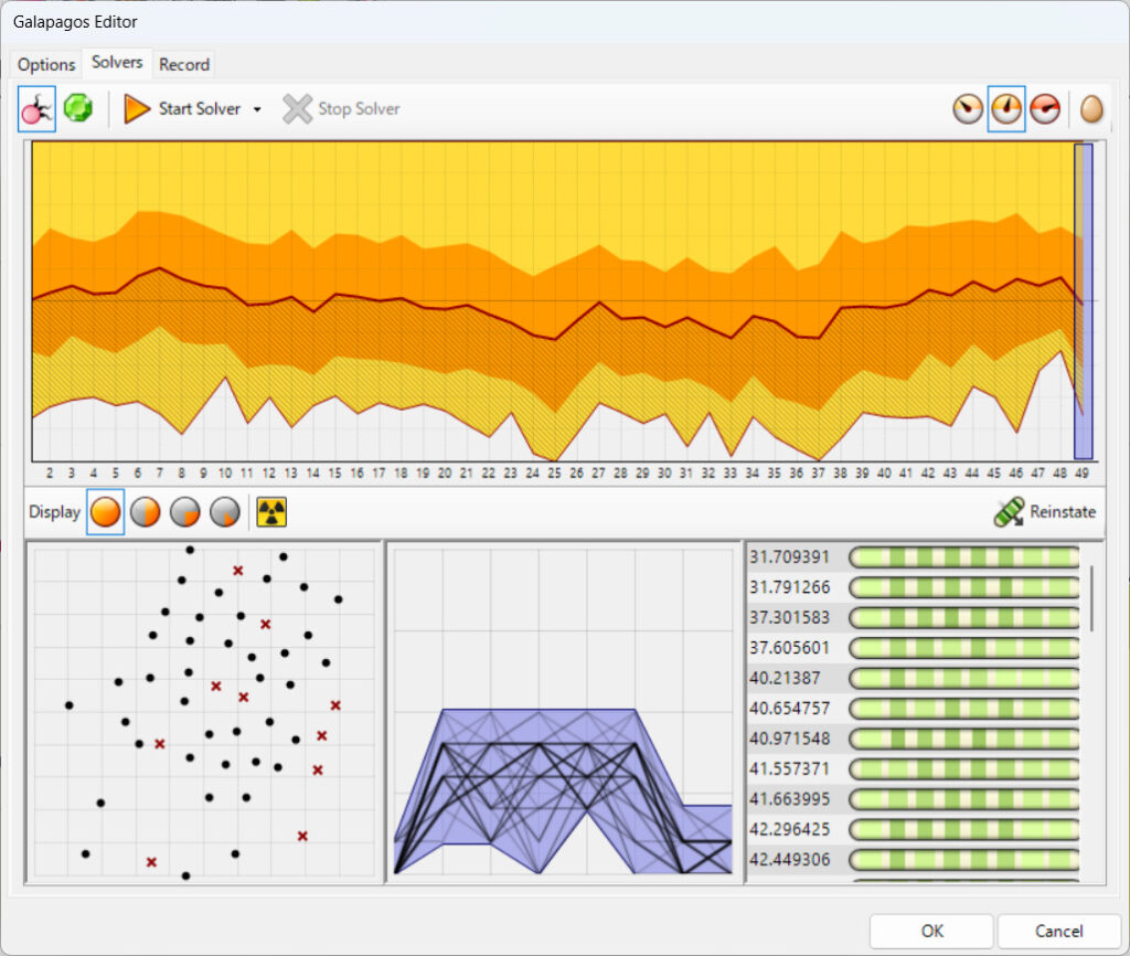
The optimization will then begin.

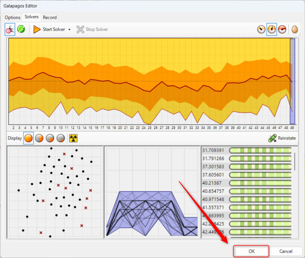
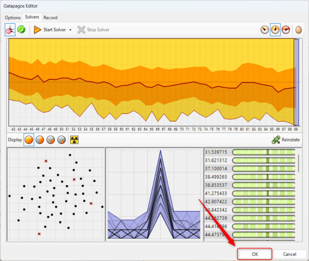
After optimization is complete, click the OK button in the lower right corner.

This completes the basic optimization.

Various Optimization Settings

Next, let’s take a look at the various optimization settings.

Galapagos has three tabs: Options, Solvers, and Record.

Options tab

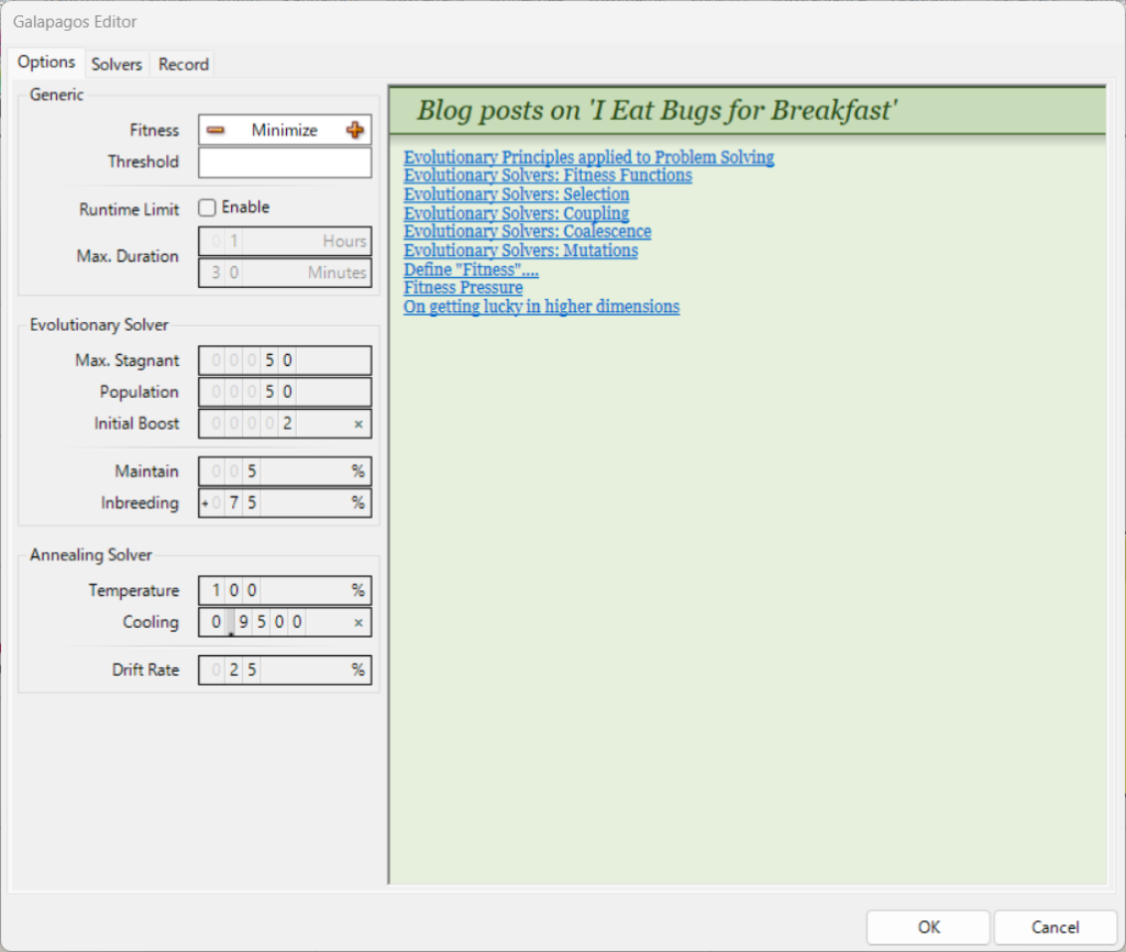
In the Options tab, you can configure general optimization settings and two types of optimization settings: Evolutionary Solver (genetic algorithm) and Simulated Annealing Slover (annealing method).

Generic

Generic offers general settings for optimization.

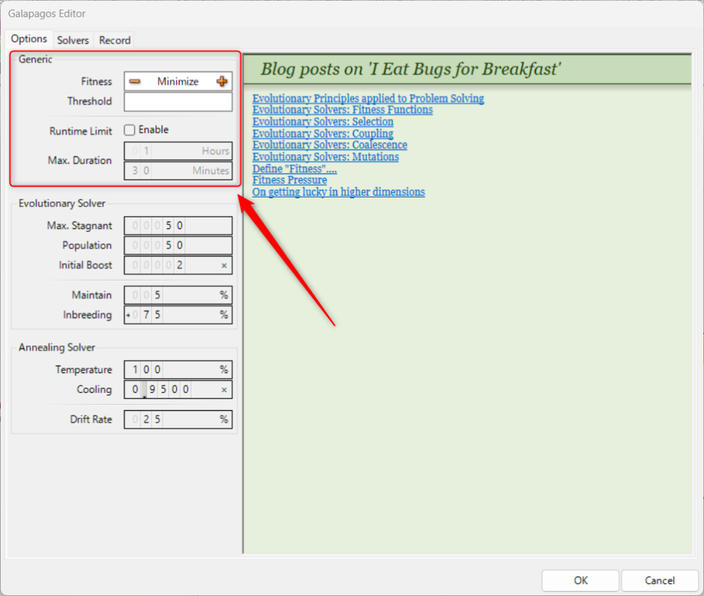
Fitness determines whether the values are optimized to maximum or minimum.

Press the + mark to optimize to the maximum of Maximize and the – mark to optimize to the minimum of Minimize.

Threshold allows you to set a threshold value.

For example, if a number can be optimized by maximizing it up to 50, but you specify 40 in Threshold, the number will not exceed 40.

Similarly, if a number can be optimized by minimizing it to 50, a Threshold of 60 will ensure that the number never falls below 60.

If you put a check mark in Enable under Runtime Limit, you can limit the time taken for optimization.

Then, in Max. Duration, set Hours to hours and Minutes to minutes to complete the time limit setting.

Evolutionary Solver

Evolutionary Solver allows you to set the optimization method of the Evolutionary Solver (genetic algorithm).

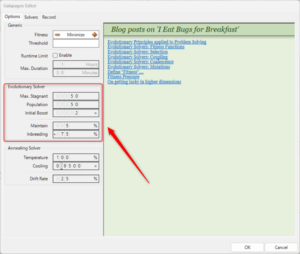
In Max. Stagnant, set the number of generations to be repeated.

If the value is 50, 50 generations will be created and the ideal individual will be selected from the 50th generation.

Population sets the numerical value for the number of individuals in one generation.

If the number is 50, 50 individuals will be generated per generation.

Initial Boost is the number of times the normal number of individuals produced in the first generation.

If Population is 50 and Initial Boost is 2, 100 individuals will be produced in the first generation (50 x 2).

The second and subsequent generations will produce 50 individuals.

Annealing Slover

Annealing Slover sets the optimization method for Simulated Annealing Slover (annealing method).

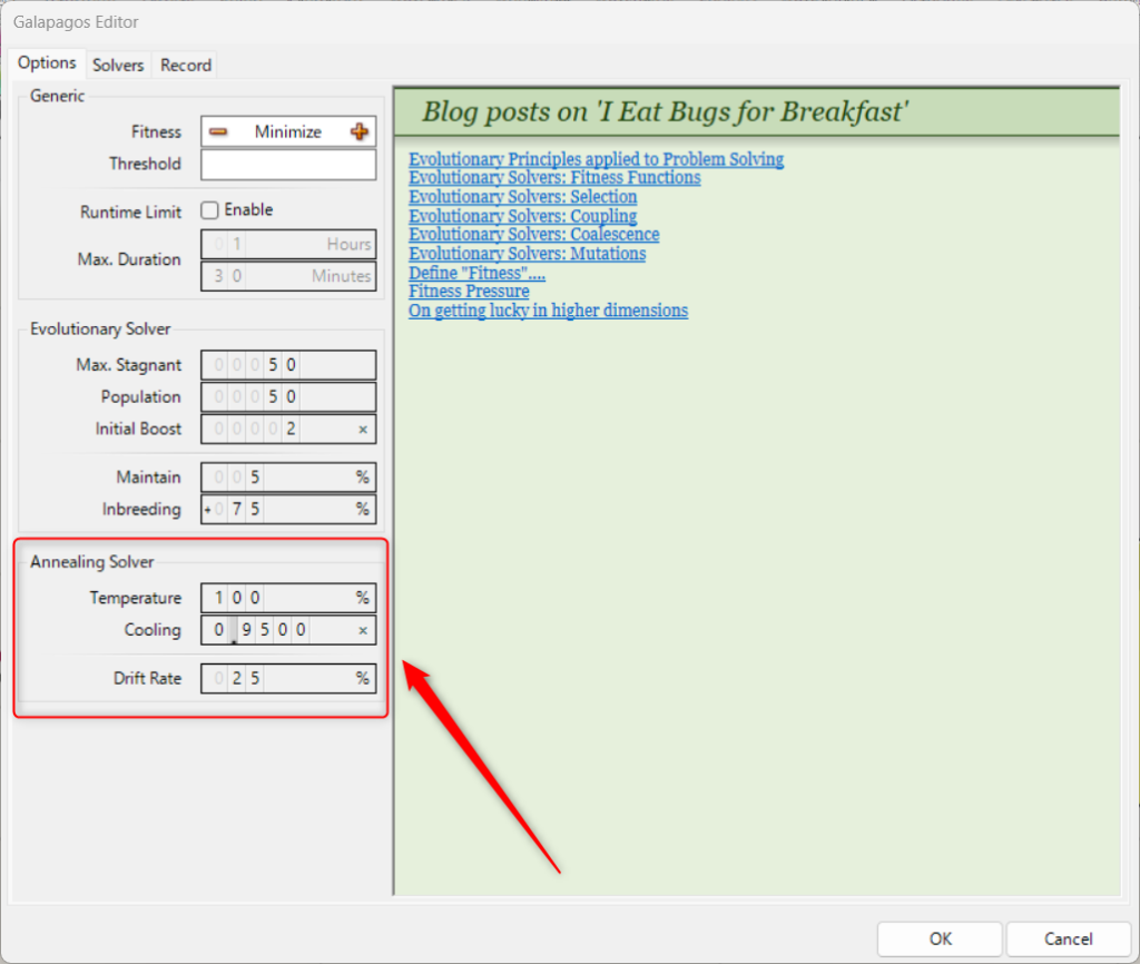
Temperature is the number of possibilities to search for other good solutions.

With temperature, the higher the value, the more molecules move, so the higher the value of Temperature, the more possibilities are explored.

Cooling is the numerical value of how much the Temperature temperature is lowered when exploring different possibilities.

The lower the Temperature temperature, the less other solutions are explored.

Therefore, the lower this ratio is, the faster the Temperature is lowered.

If Temperature is 100 and the number is 0.95, then 100 x 0.95 equals 95, 95 x 0.95 equals 90.25, and so on.

Drift Rate is the numerical value of the rate at which the parameter variable is changed.

If the Drift Rate is 25%, one process will change 25% of the variables in a quarter.

URL link to the I Eat Bugs for Breakfast blog page

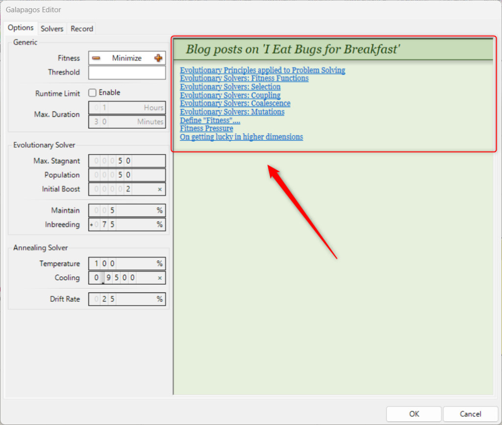
In the right half of the page, you will find the URL link to the I Eat Bugs for Breakfast blog page, which describes the Galapagos algorithm in English.

Solvers Tab

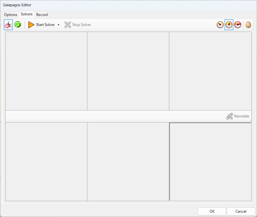
The Solvers tab allows you to run optimizations and configure settings related to their execution.

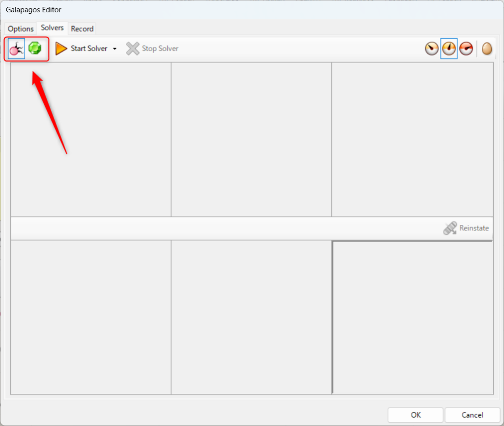
The two icons in the upper left corner allow you to select the optimization method.

On the left is the Evolutionary Solver (genetic algorithm).

On the right is the Simulated Annealing Slover.

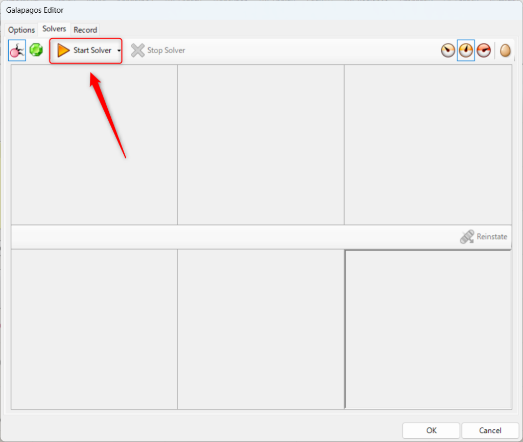
By pressing Start Solver, you can start the optimization.

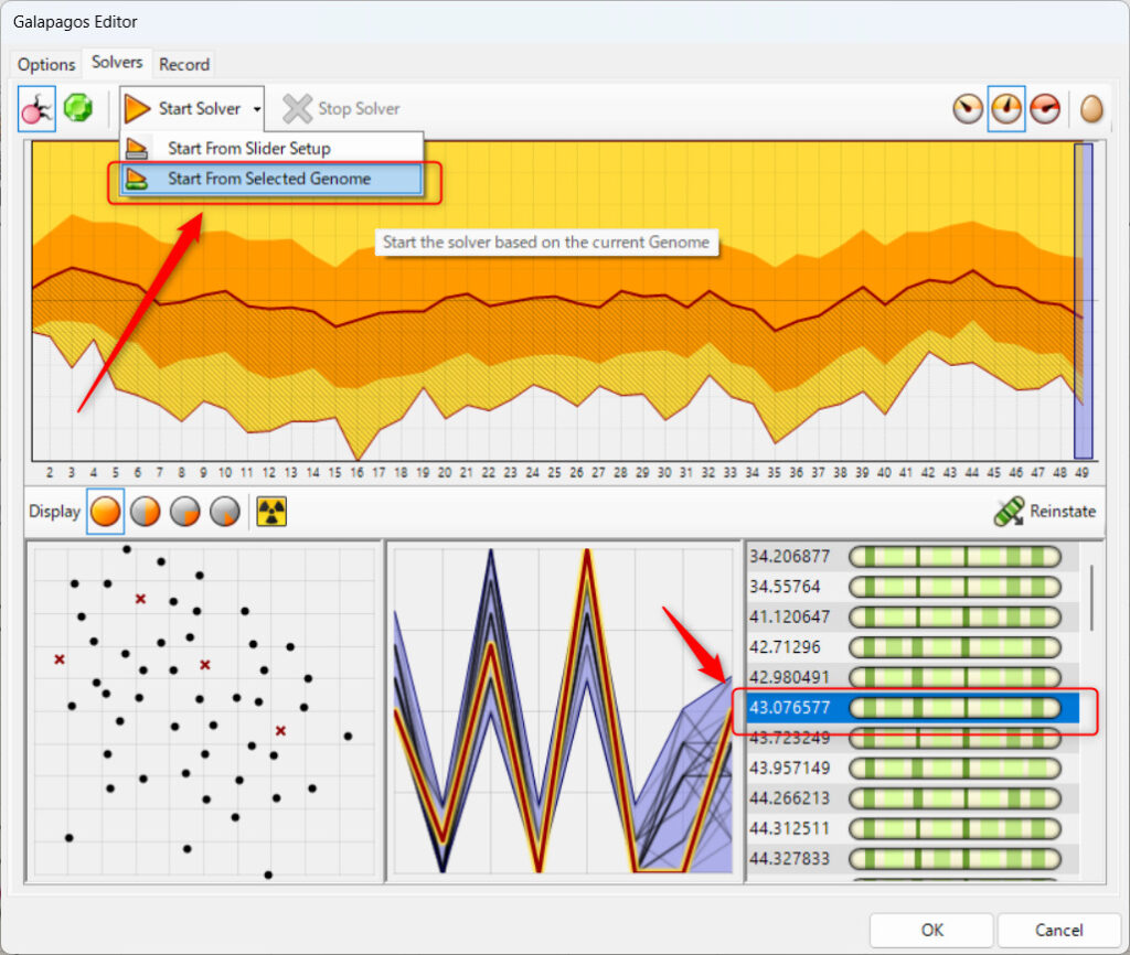
The basic option is Start From Slider Setup, but you can select Start From Selected Genome if you have selected a once-optimized result in the lower right corner.

In this case, the optimization can be performed again based on the selected results.

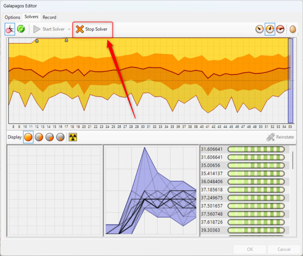
Pressing “Stop Slover” allows you to stop the optimization in progress.

If you stop, you can use the optimization results up to the point where you stopped.

The icon in the upper right corner allows you to set the display of the individual files in the process of optimization on the Rhinoceros.

In the case of the leftmost icon, all the individuals in the process of optimization are displayed on the Rhinoceros.

With the second icon from the left, only the best individuals will be displayed on the rhinoceros.

The third icon from the left will not show any individuals on the rhinoceros.

The rightmost egg icon is About, which should be about optimization, but as of September 2024, nothing happens.

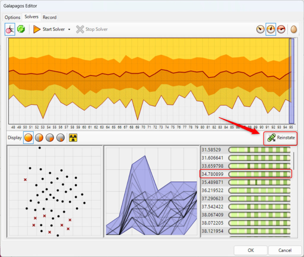
After optimization is complete, Reinstate can be used.

Select the superior individual shown on the right and press Reinstate, and the result will be reflected in the Grasshopper parameters.

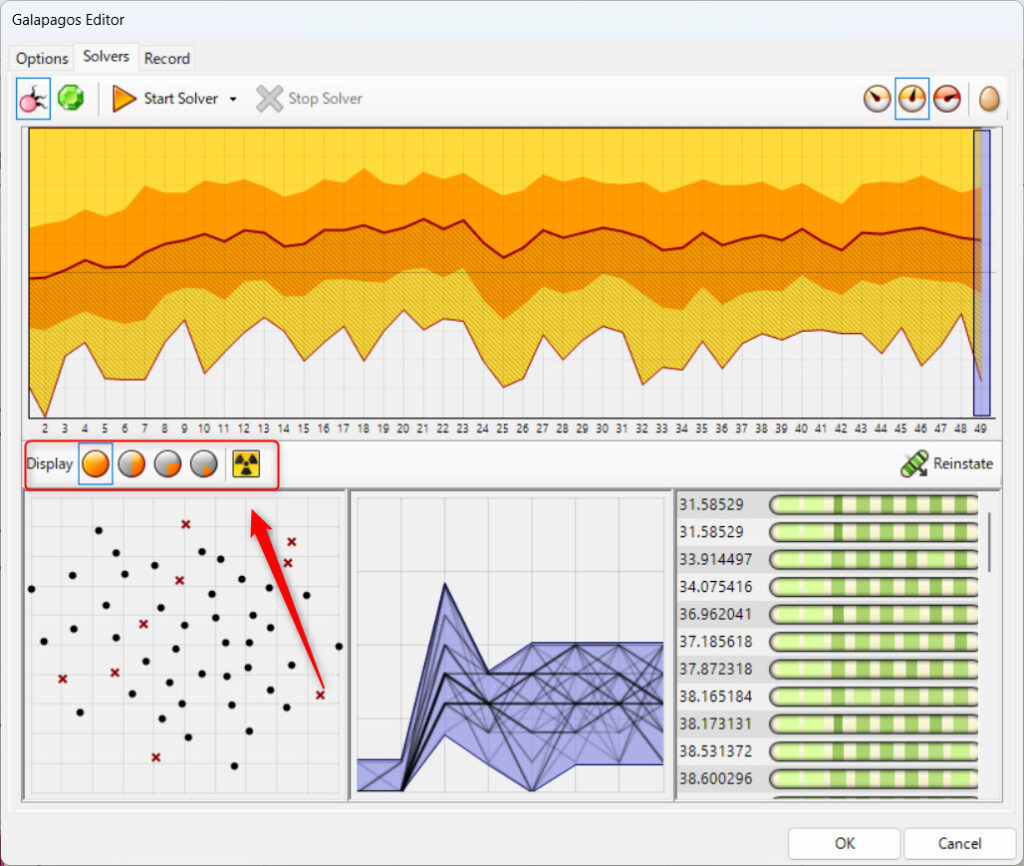
The red box above is an icon that appears only in the Evolutionary Solver (Genetic Algorithm).

Select the leftmost icon to see all the individuals that appeared.

If you select the second icon from the left, you will see only the top 50% of the individuals.

Selecting the third icon from the left will show only the top 25% of the individuals.

Selecting the fourth icon from the left will show only the top 10% of individuals.

Clicking on the rightmost icon during optimization allows you to create new mutations and explore new possibilities.

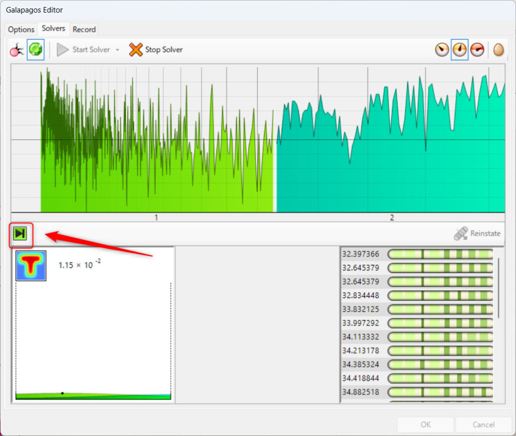
The red framed area above is an icon that appears only for Simulated Annealing Slover (annealing method).

Clicking it during optimization will skip that stage of optimization and proceed to the next stage of optimization.

Record Tab

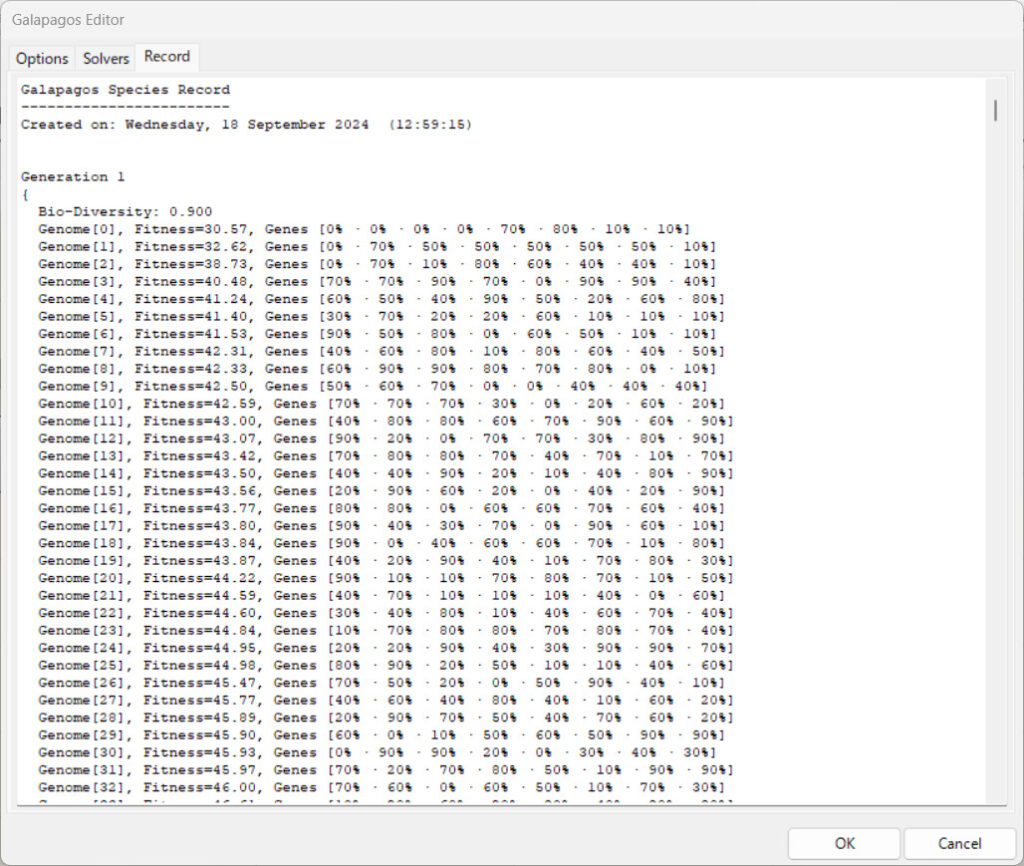
The Record tab displays the optimization performed after the optimization is complete.

Example of Use

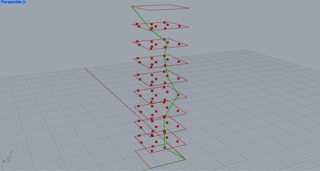
As an example, a point is randomly created on the 2nd~8th floor of a 10-story building, and the shortest distance to the diagonal between the 1st floor and the 10th floor is optimized.

Preliminary Preparation for Optimization

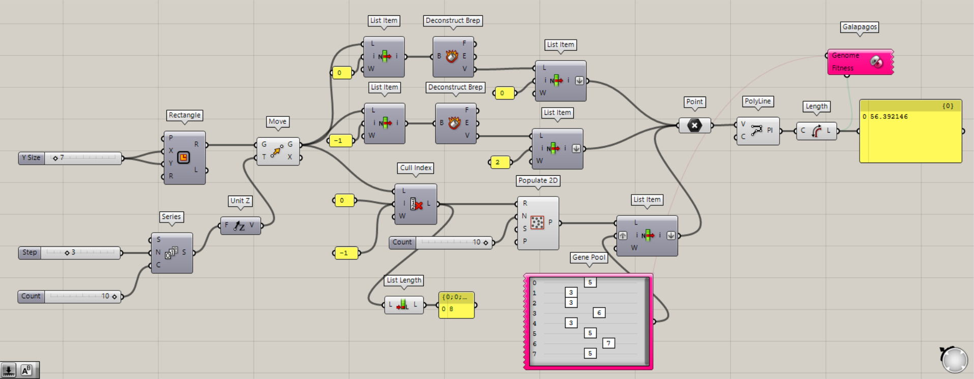
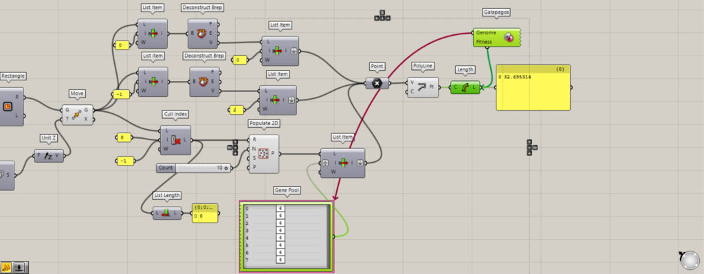
Overall components: 1) Rectangle 2) Series 3) Unit Z 4 ) Move 5) Cull Index 6) Populate 2D 7) List Length 8) Gene Pool 9) List Item 10) Deconstruct Brep 11 ) Point 12) Polyline 13) Length 14) Galapagos

First, create 10 floors.

First, create a square using Rectangle.

This time, we put the number 7 in the X and Y terminals to create a 7 x 7 square.

Then, we create a sequence of isosceles numbers in Series.

Enter the number 3 into the Series(N).

Enter the number 10 into the Series(C).

This creates 10 numbers that increment by 3 from 0.

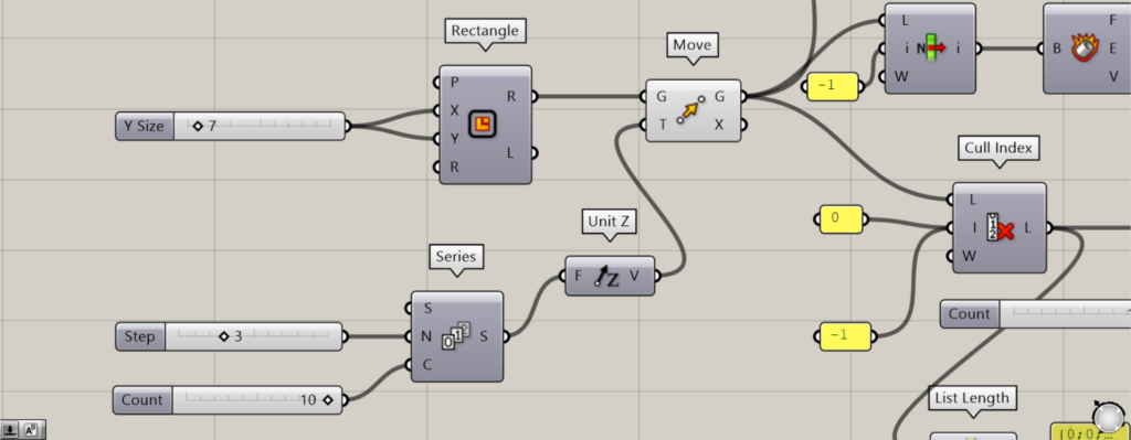
Then connect the Series to Unit Z.

Then connect the Rectangle(R) to the Move(G) and connect Unit Z to the Move(T).

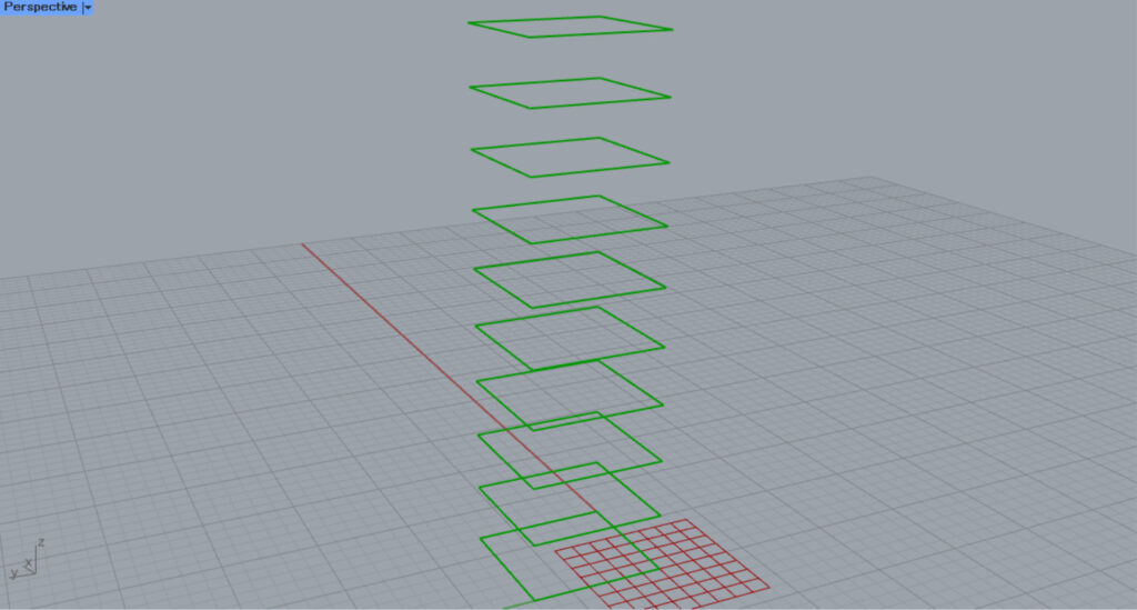
This creates 10 squares with an interval of 3 directly above the Z-axis.

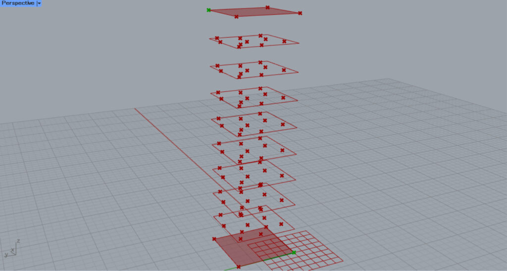
Next, we will randomly create points on the 2nd to 8th floors.

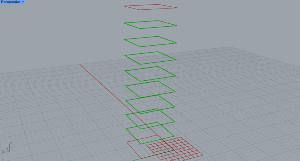
Connect the Move(G) to the Cull Index(L).

In addition, input 0 and -1 to the Cull Index(i).

Then, the first and last data, the 1st and 10th floors, are deleted, and only the 2nd to 8th floors are extracted.

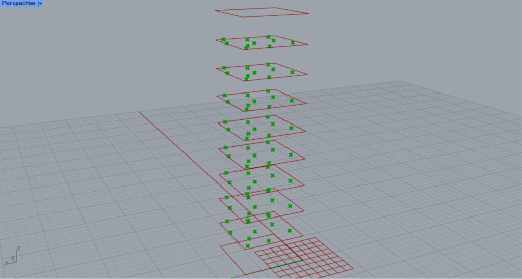
The Cull Index is then connected to Populate 2D(R).

Enter the number of points in the Populate 2D(N).

In this case, we entered 10.

Then, 10 points were randomly generated on each floor.

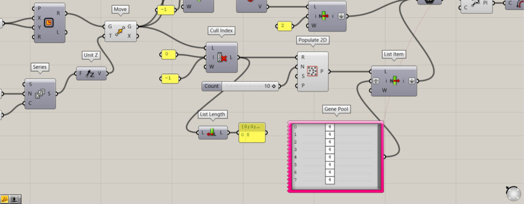
After that, connect Populate 2D to the List Item(L).

Then, connect Gene Pool to the List Item(i).

Also, connect Cull Index to List Length.

The number of data in the Cull Index can then be checked.

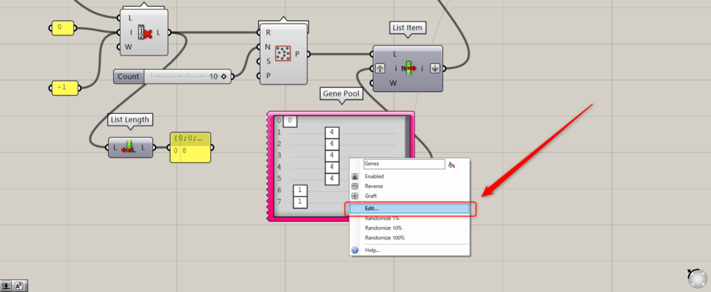
At this time, set the Gene Pool settings.

Right-click on the Gene Pool and select Edit.

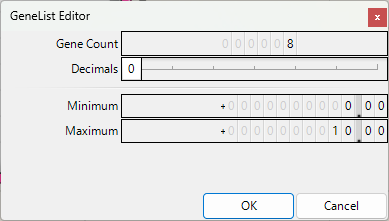
The Gene Pool settings window will appear.

In Gene Count, enter the number of 8 you confirmed in List Length.

In Decimals, specify the decimal point unit.

For Minimun, set it to 0, and for Maximum, set it to 10.

Then, we were able to set variables 0~10 for each of the 8 data individually.

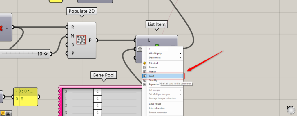
When connecting the Gene Pool to the List Item(i), right-click on the List Item(i) and select Graft.

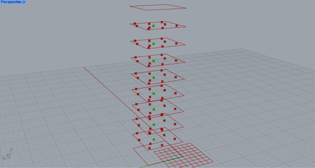
Then, one point on each floor will be selected like this.

This selected point can be changed by changing the variable.

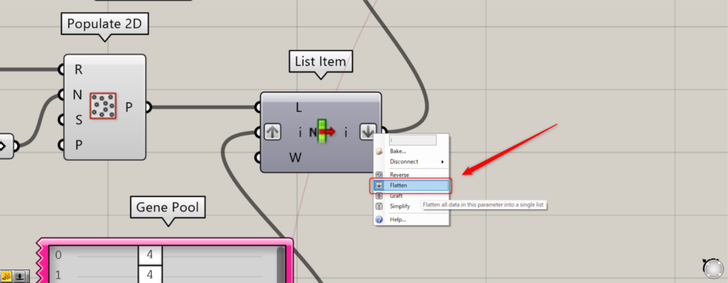
Also, right click on the right terminal of the List Item and set it to Flatten.

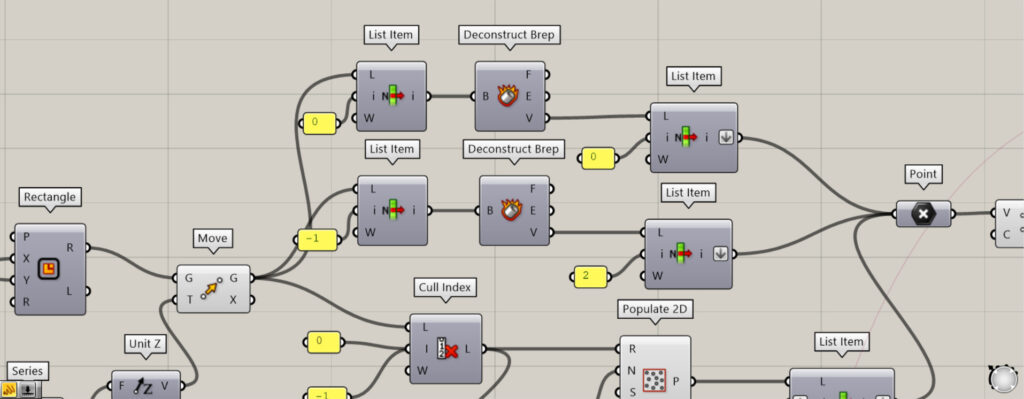
Next, we will go back a bit and get the points on the first and tenth floors.

Connect the Move(G) to the two List Item(L).

In addition, input 0 to the first List Item(i) and -1 to the second.

Then, only the first and last data, the first and tenth floors, can be extracted.

Then, connect the List Item to the two Deconstruct Brep, respectively.

The square is then deconstructed and the vertices can be retrieved.

Then, connect the two Deconstruct Brep to the two new List Item(L).

Input 0 to the first List Item(i) and 2 to the second.

Now we have obtained the points at the diagonal positions of the first and tenth floors.

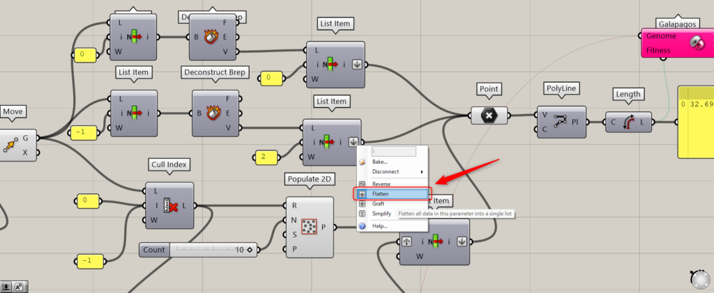
At this point, right-click on the right terminals of the two List Items and set them to Flatten.

Then, connect the three List Items to the Point.

At this time, be careful about the order in which they are connected.

The order should be: List Item with i terminal 0 →List Item inGenePool → List Item with -1.

The reason for this is that you want the order to be from the first floor to the tenth floor when you connect them with a line.

After that, connect the points to the Polyline(V).

Then, connect the Point to Polyline(V) to create a line connecting one point on each floor.

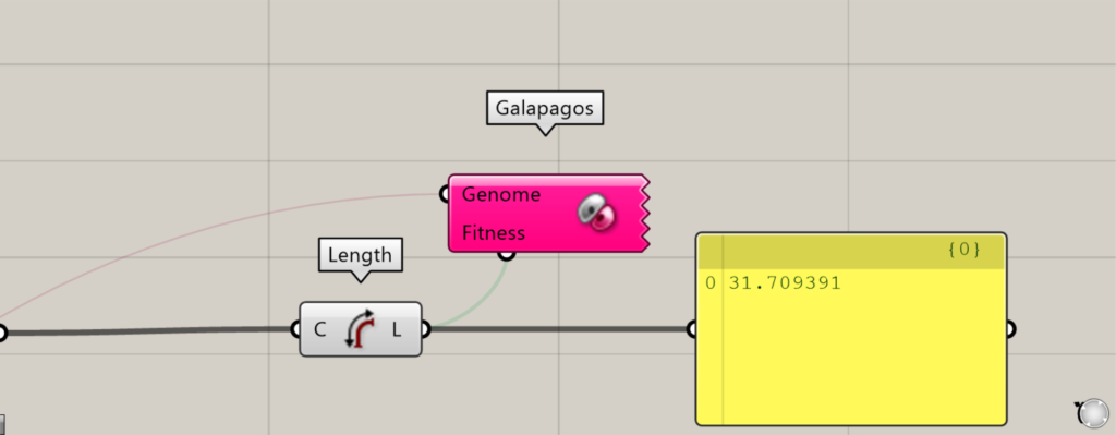
Connect Polyline to Length to get the length of the line.

Finally, connect the Fitness terminal of Galapagos to Length and the Genome terminal to Gene Pool.

This completes the preliminary optimization preparation.

Performing Optimization

Perform the actual optimization.

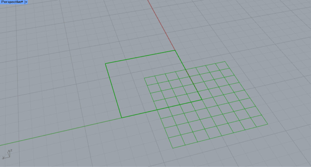
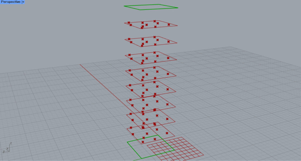
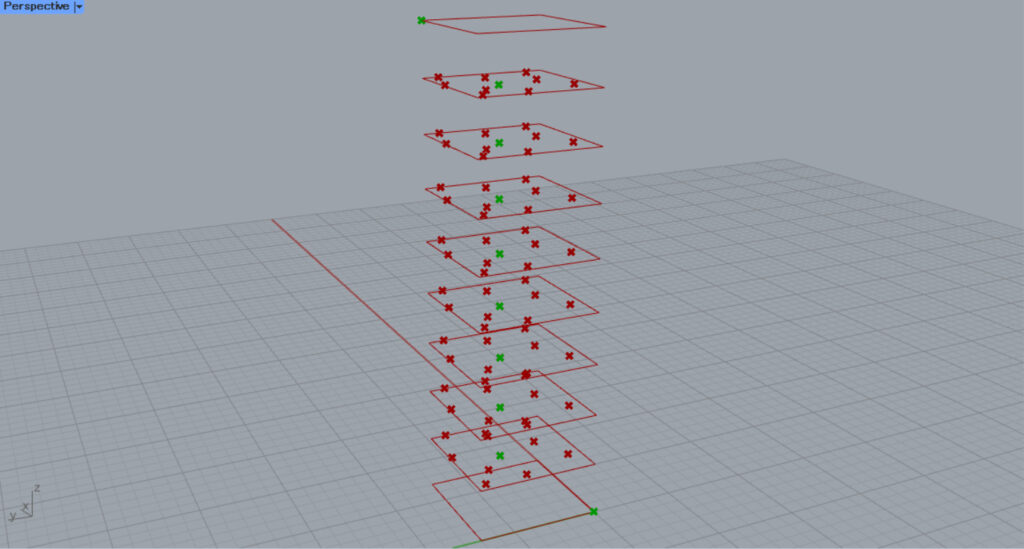
The image above shows the pre-optimization state with appropriate variables.

Optimization is performed so that this line is shortened by the shortest distance.

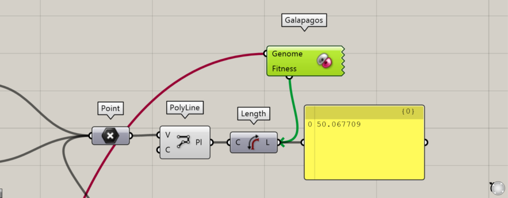
The length of the line at this stage is about 50.

To optimize, double-click on Galapagos.

To minimize the value, click on the – icon and set it to Minimize.

Select the Slovers tab.

This time, select the Evolutionary Solver (genetic algorithm) optimization method.

After selecting the optimization method, press “Start Solver” to run the optimization.

The optimization has now started.

After the optimization is complete, press the OK button in the lower right corner.

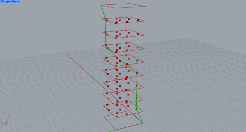
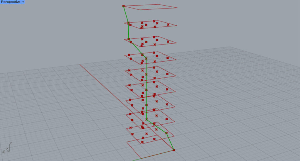
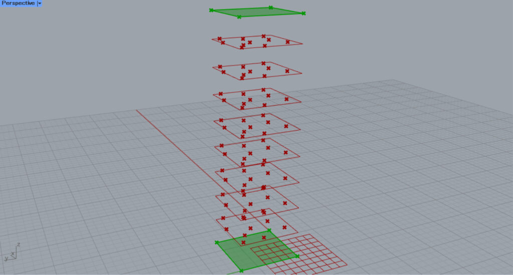
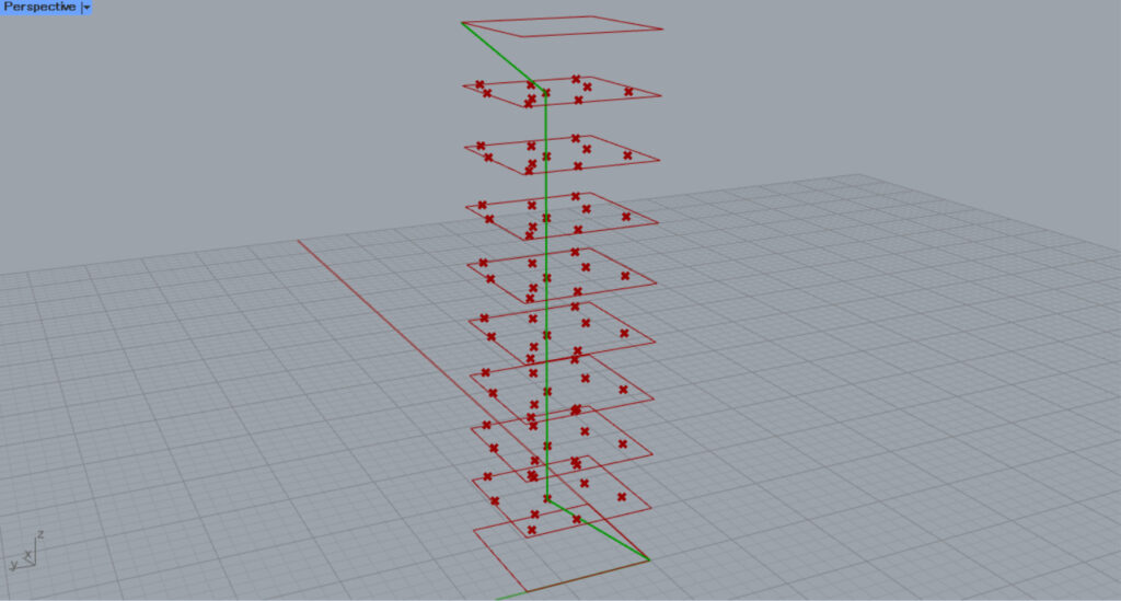
The result of the shortest distance is shown in the image above.

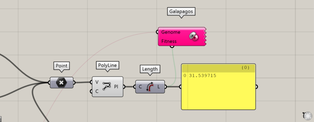
The line distance is also about 31, which is very much smaller than the previous result of about 50.

Points to keep in mind

Here are a few things to keep in mind when using Galapagos.

When optimizing to a specific number

By default, Galapagos can only optimize numbers to the minimum or maximum.

Therefore, if you want to get close to a certain number, you will need to do some programming or configuration.

Basically, by setting a threshold value in Threshold, you can make sure that the value will not be exceeded.

Also, if you want the number to be 0, but it continues to be optimized to – permanently, you can use Absolute to make it absolute, in addition to setting the threshold, so that it will not be optimized below 0.

In some cases, using a formula to adjust the value to be optimized can also be useful.

Devise ways to make the system less heavy.

When optimizing with Galapagos or other software, it is important to make sure that the model to be optimized is not too heavy.

The heavier the model is, the longer the processing time will be.

In this use case, each floor is created, but only in the state of line data in order to lighten the weight, avoiding the creation of a three-dimensional model.

In this way, simplifying or reducing the model can reduce the time required for optimization.

After optimization, we recommend creating the detailed part of the model.

The process can be stopped in the middle.

Even with various efforts, the processing time for optimization can be very long.

Although it depends on the progress of the project, etc., in some cases it is effective to stop optimization in the middle and adopt the optimization status at that point, instead of waiting for the process to be completed to the end.

Consider multiple patterns.

Optimization does not always result in the best ideal outcome.

Therefore, it is recommended to perform optimization multiple times and look at different patterns before choosing the result to use.

List of Grasshopper articles using Galapagos component↓