[Grasshopper] How to use Point Charge to create magnetic field data from points

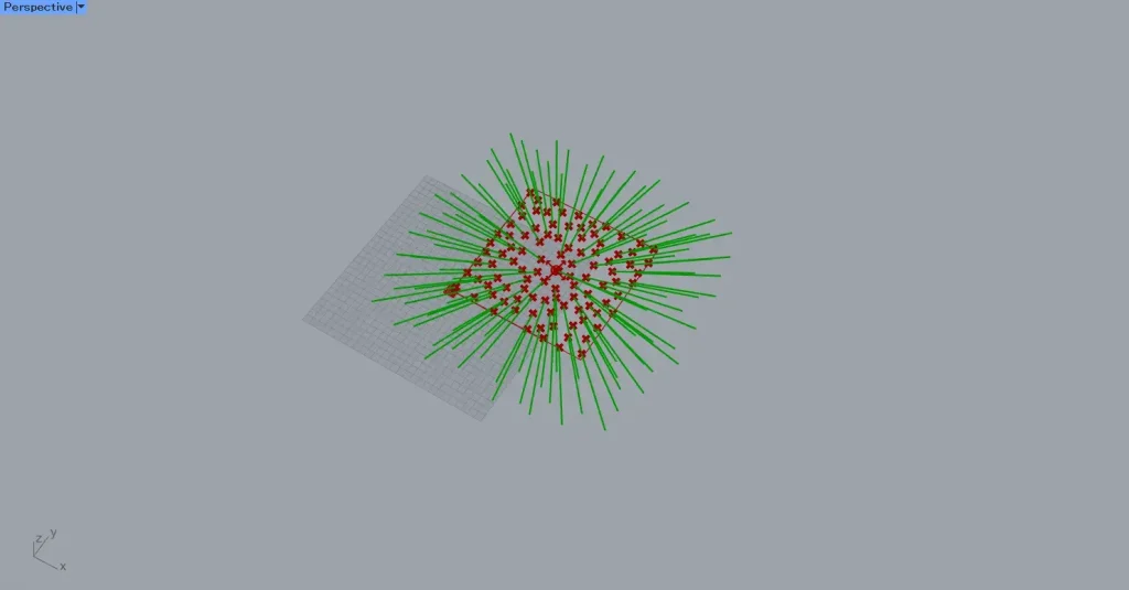
This article explains how to use Point Charge to create magnetic field data from points.

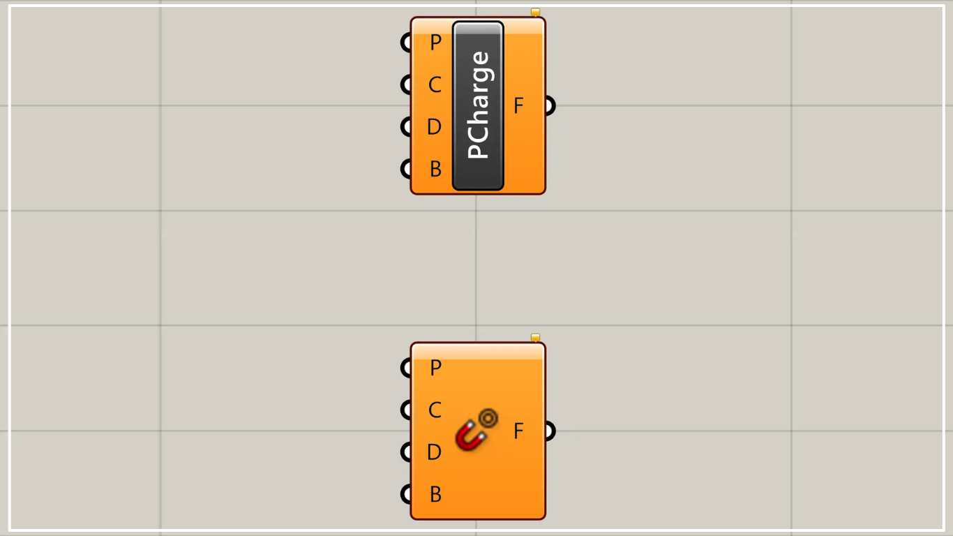
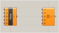
On the Grasshopper, it is represented by either of the two above.

Create magnetic field data from points

Using Point Charge, you can create magnetic field data from points.

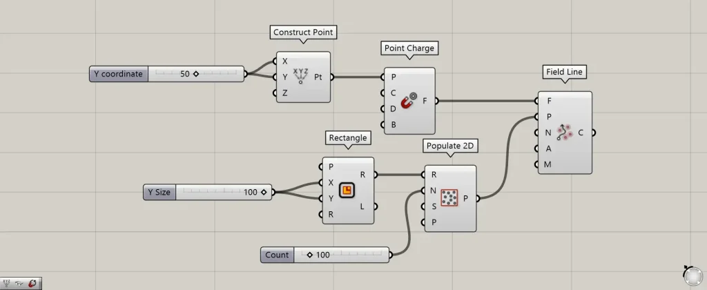
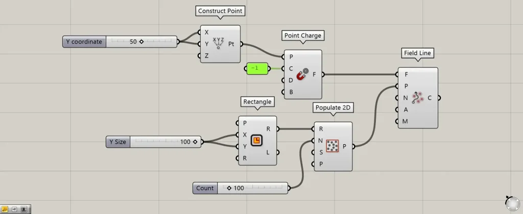
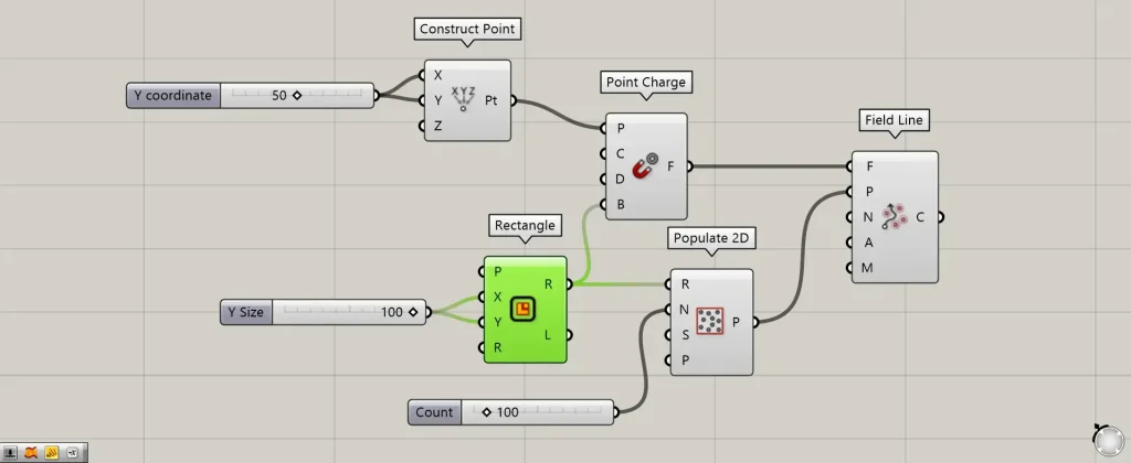
Components Used: ① Construct Point ② Point Charge ③ Rectangle ④ Populate 2D ⑤ Field Line

As a first example, we will create magnetic field data using the specified point data and visualize that magnetic field data.

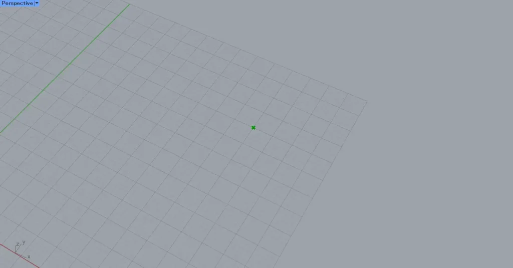
First, enter 50 into the Construct Point(X and Y).

Then, a point was created at the coordinates 50,50,0.

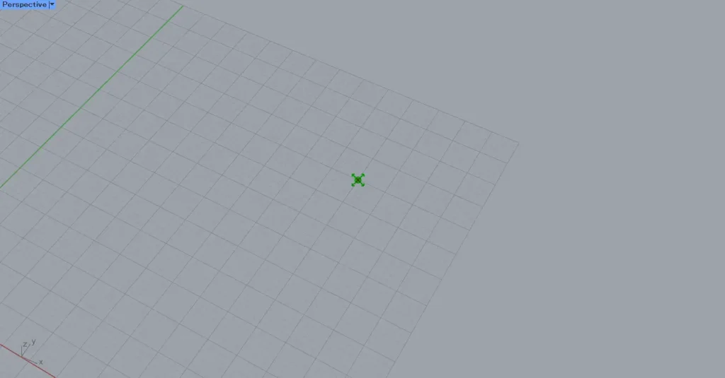
Then, connect the Construct Point to the Point Charge(P).

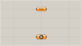
Then, a magnetic field is created as shown in the image above.

In the initial state, an arrow pointing outward from the point is displayed.

This means that the magnetic field exerts its influence outward.

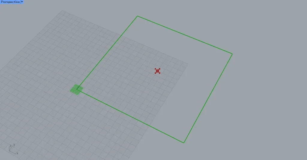
Let’s visualize the magnetic field.

Enter 100 into the Rectangle(X and Y) to create a 100×100 rectangle.

Next, connect Rectangle(R) to Populate 2D(R).

Then, enter the number of points to generate randomly into Populate 2D(N).

This time, we entered 100.

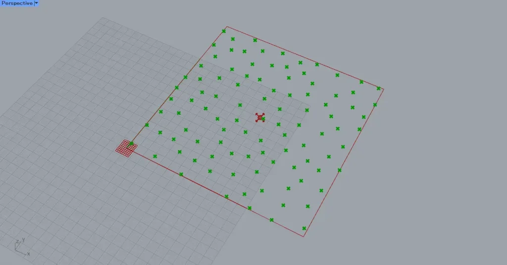
Then, 100 points were randomly created within the rectangle.

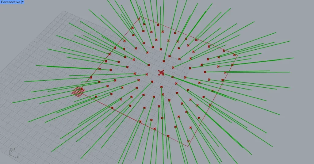
Then connect the Point Charge to the Field Line(F).

Additionally, connect Populate 2D to the Field Line(P).

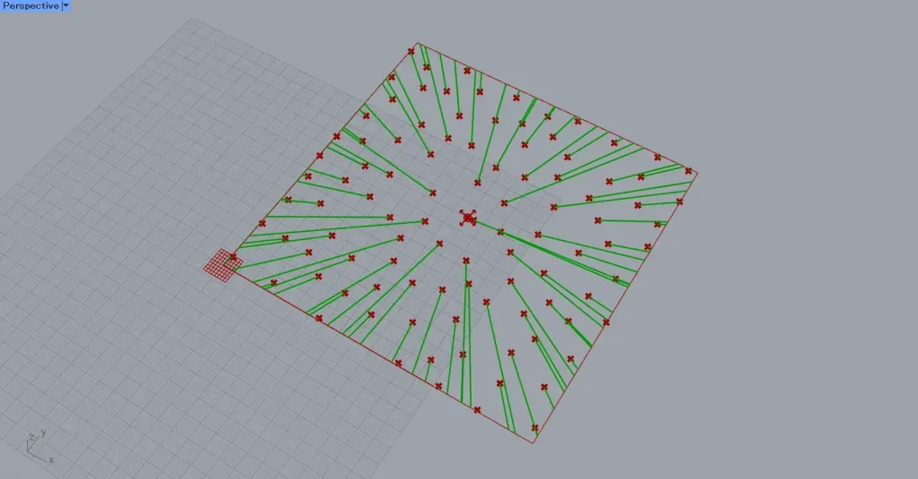
Then, lines were created from the points we made, reflecting the influence of the magnetic field.

In this case, since the magnetic field is located at the center of the square, lines are drawn away from the center.

In this way, a magnetic field can be created from point data.

At the Point Charge(C), you can specify the strength and direction of the magnetic field’s magnetic force.

Entering a negative value into the Point Charge(C) creates a magnetic field that pulls objects toward the specified point.

For example, let’s input the value -1 into the Point Charge(C).

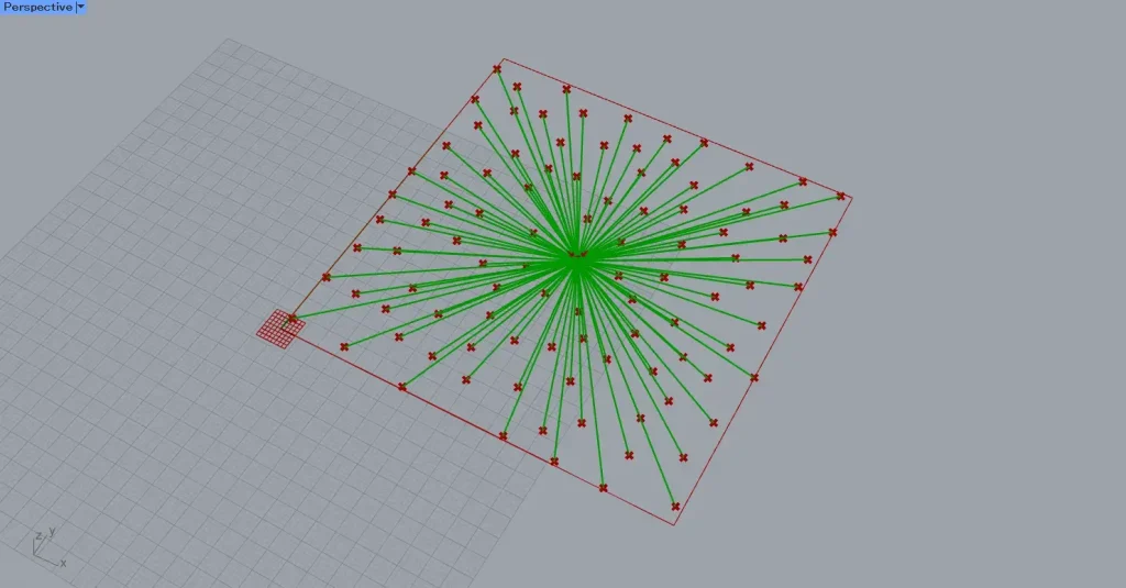
Then, lines are drawn as if drawn toward the specified point, and you can see that the direction of the magnetic field has reversed.

Looking at the point specified as the magnetic field location, you can see that the arrow at the point is pointing inward, confirming that it is reversed.

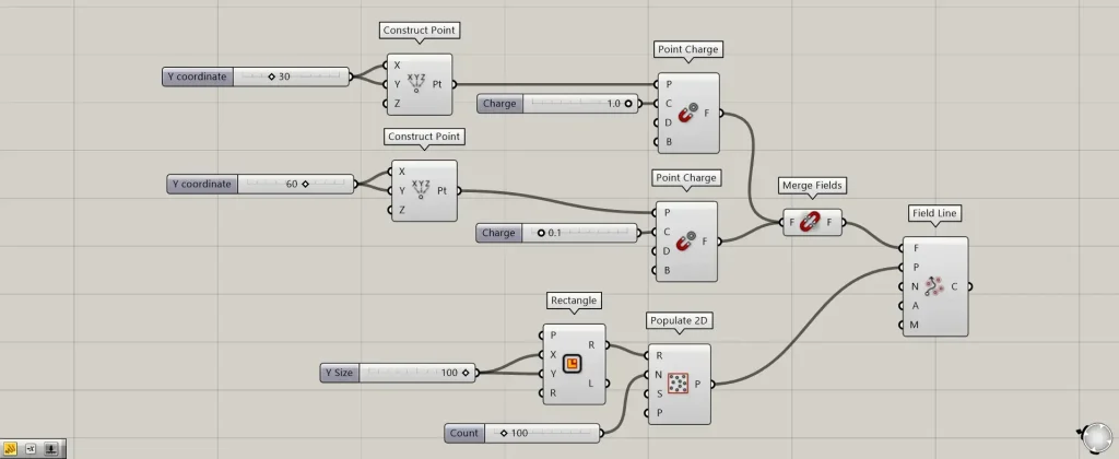
Additional Components: ① Merge Fields

To verify the strength of the magnetic force, two points were specified.

One coordinate is set at 30,30,0, and the other is created at 60,60,0.

And while each one creates a magnetic field using Point Charge, the strength of the Point Charge(C) is being altered.

The first value is set to 1.0, and the other is set to 0.1.

Then, two point charges are merged into a single magnetic field using merge fields.

Then, you can see the difference in the strength of the magnetic force between the two points.

The magnetic field in the lower left has a value of 1.0 entered, and the one in the upper right has a value of 0.1 entered.

Therefore, we can see that the magnetic force is stronger in the lower left area.

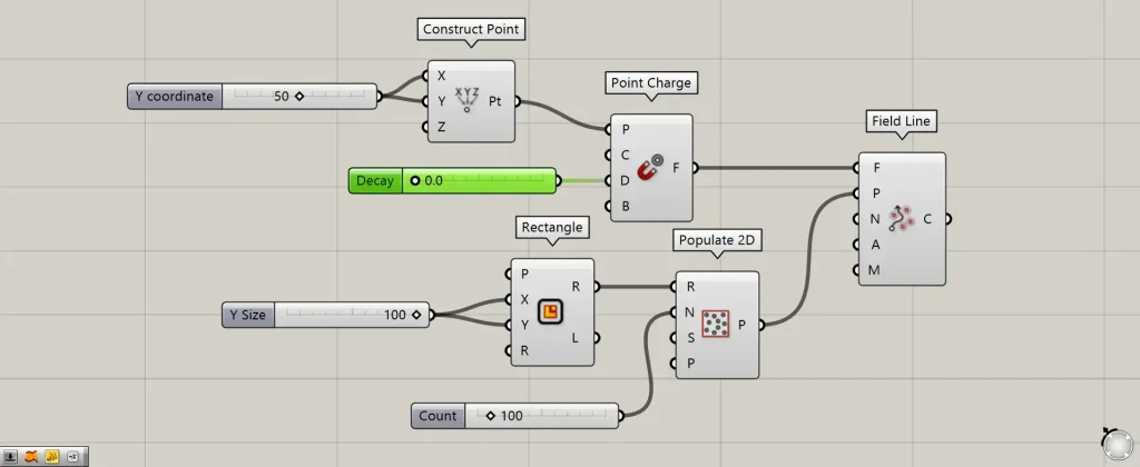
With the D terminal, you can set the range of influence by specifying the magnetic force attenuation value.

The larger the number, the smaller the range of influence of the magnetic field.

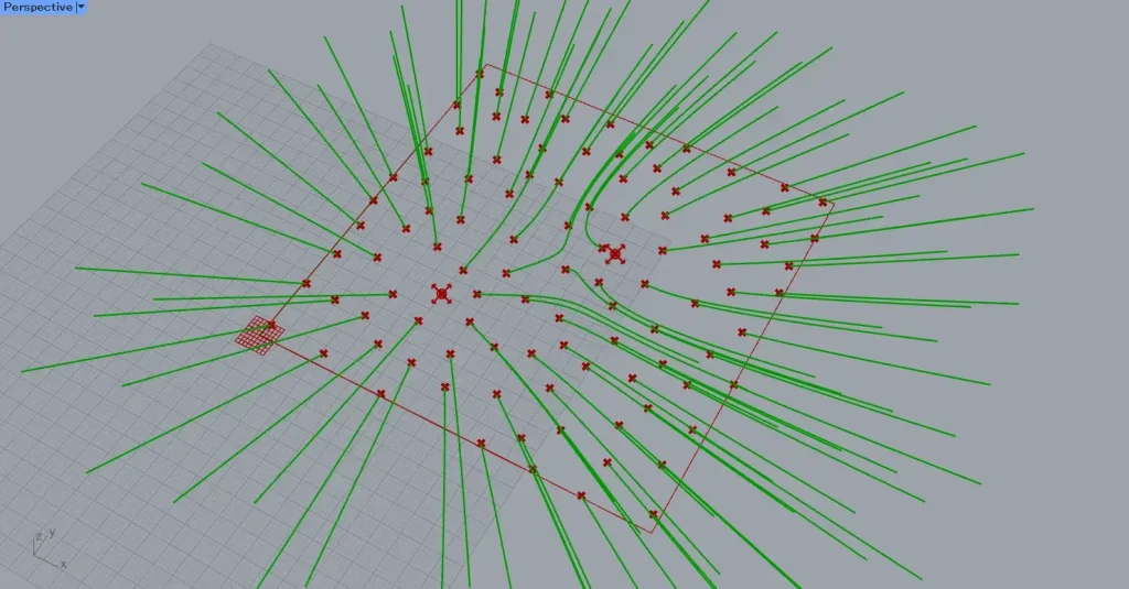
Here is the D terminal reading at 0.

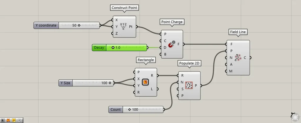
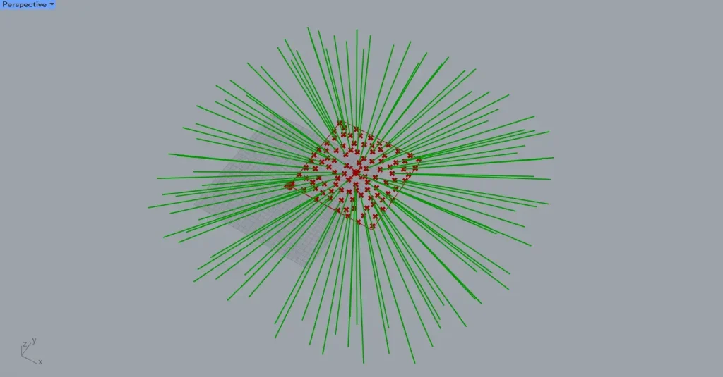
I’ll change the value of terminal D to 1.

Then, the magnetic field’s influence range decreased.

In this way, you can also adjust the range of influence of the magnetic field.

By connecting object data to the B terminal, you can also apply the magnetic field’s influence only within that object.

This time, we will connect the Rectangle(R) used for the rectangle data when creating random points.

Then, the magnetic field was reflected only within the specified rectangle.

List of Grasshopper articles using Point Charge component↓