[Grasshopper] Analysis of running water such as rainwater

In this article, we will learn how to analyze running water such as rainwater in Grasshopper.

Model Image

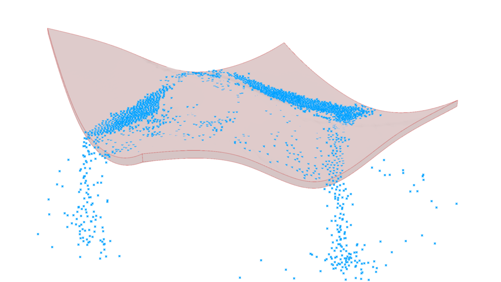
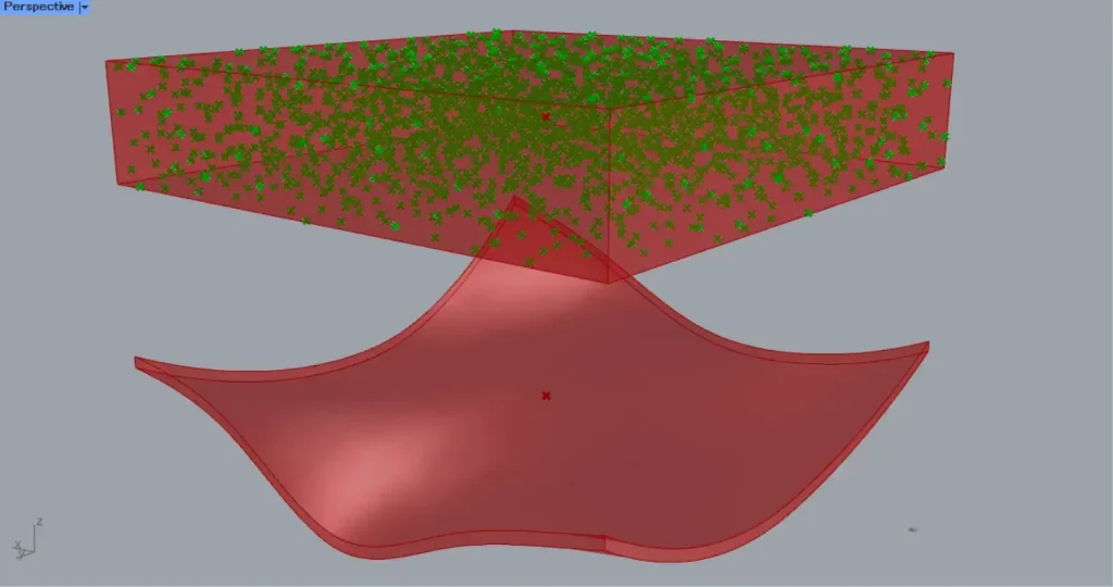
The image above shows the actual analysis being carried out.

Click here to download the Grasshopper file

Please refer to the Terms of Use regarding the use of downloadable data.

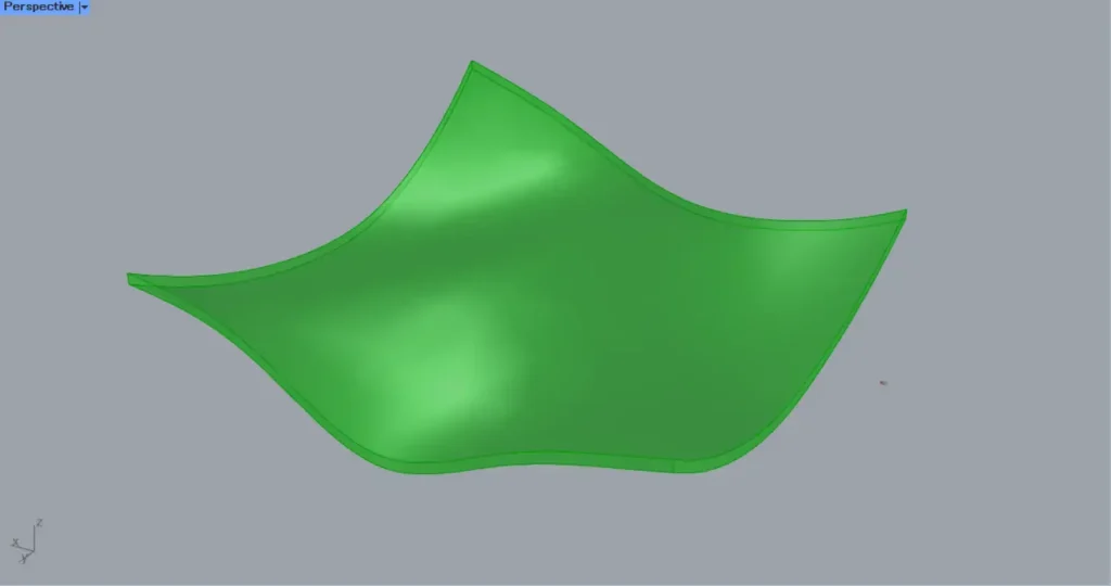
Model used in this project

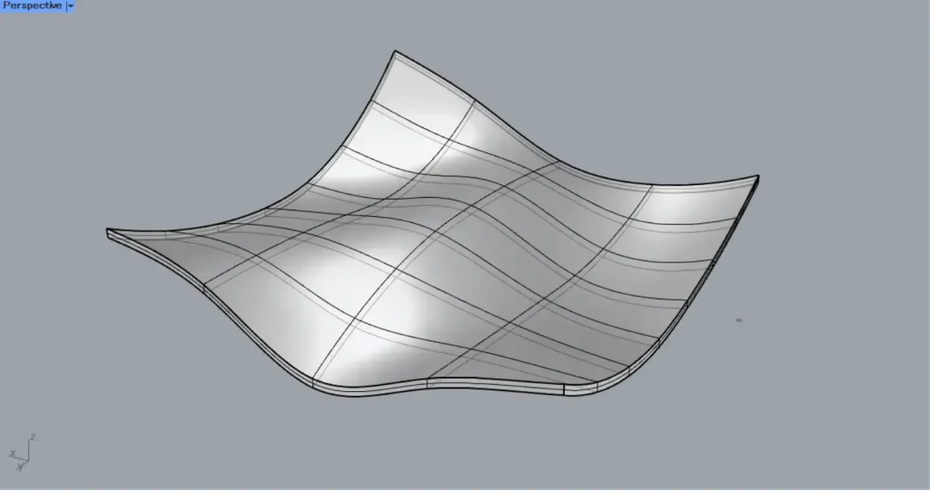
For this example, we will use the solid model on the rhinoceros in the image above.

We will proceed with the model as a roof, but of course the same analysis can be done for terrain, etc.

Grasshopper recipe

This programming uses Kangaroo2, which is standard on Rhino 6 and later.

If it is not installed, please install it.

Click here to download Kangaroo2 before Rhino6.

If you are using Rhino 6 or later, you do not need to install this software.

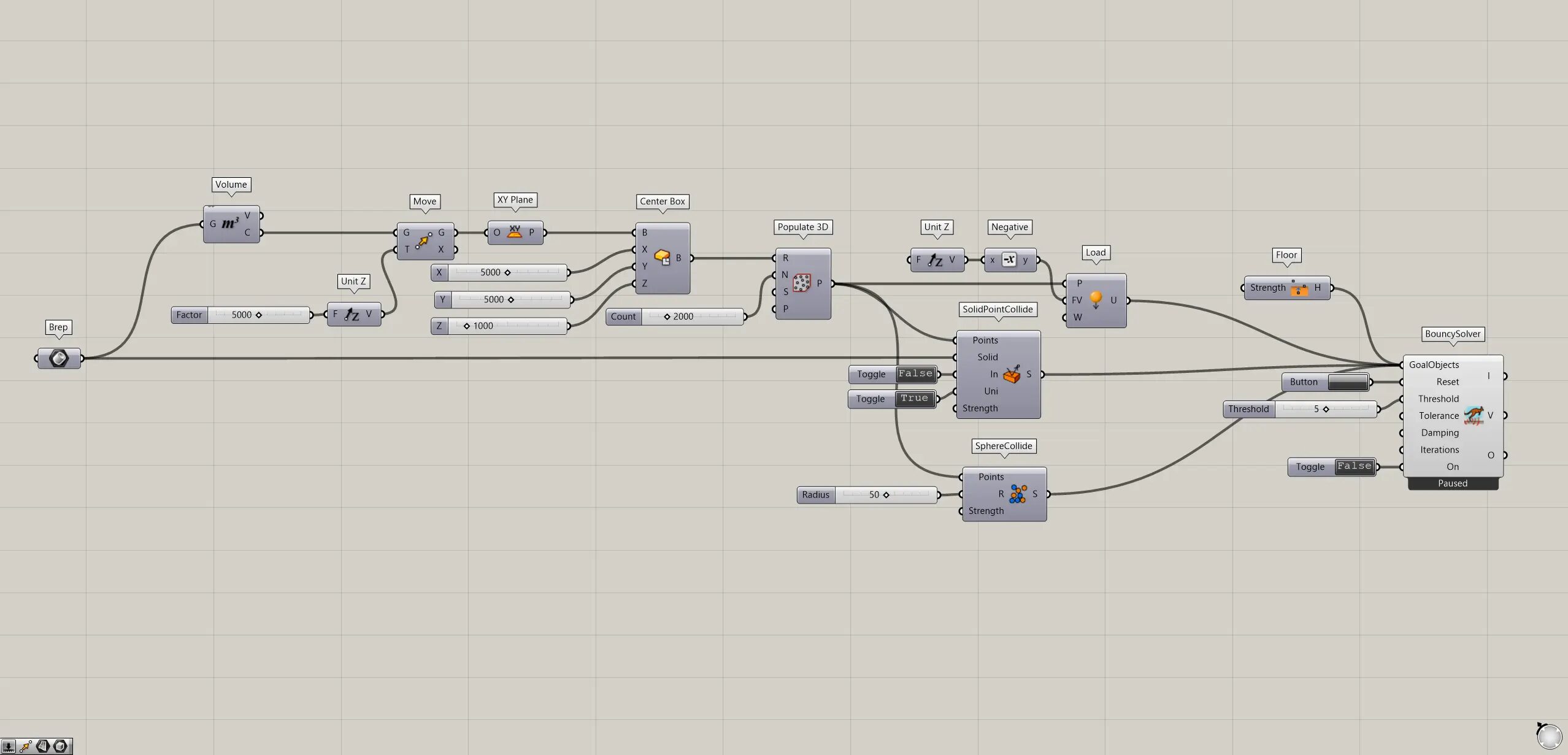
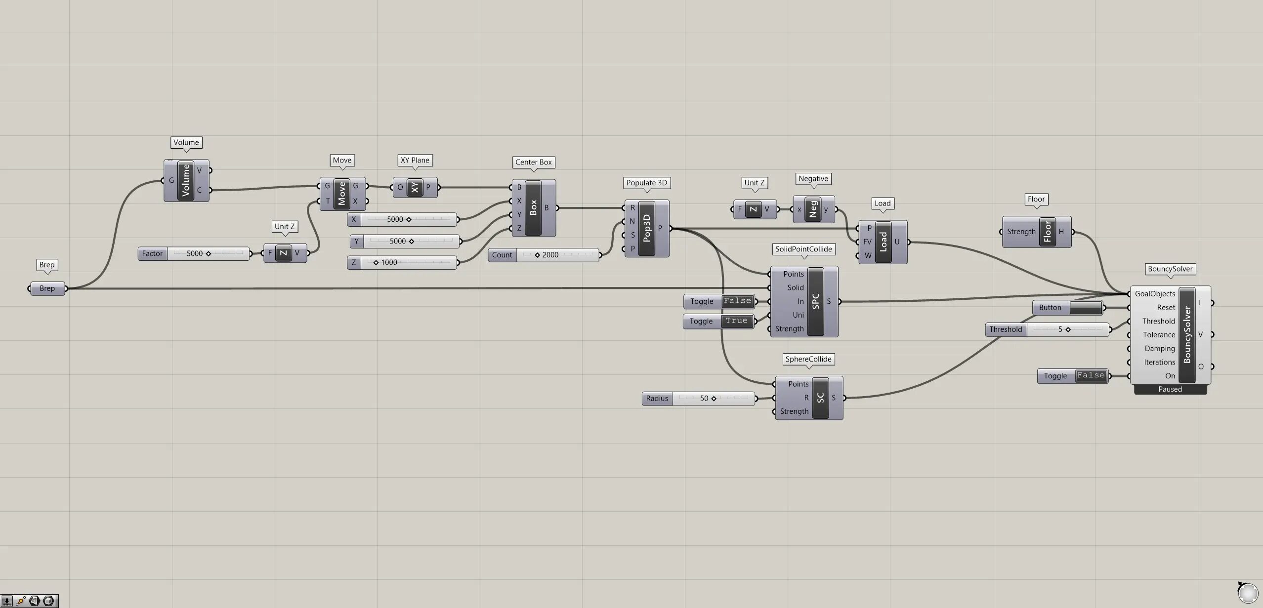
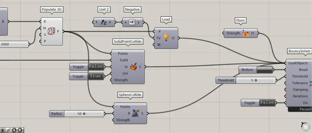
①Brep ②Unit Z ③Move ④XY Plane ⑤Center Box ⑥Populate 3D ⑦SolidPointCollide ⑧Boolean Toggle ⑨SphereCollide ⑩Negative ⑪Load ⑫Floor ⑬Button ⑭BouncySolver

Create multiple points to replace water

First, we will create multiple points that will take the place of water.

First, the model on the rhinoceros is stored in a Brep.

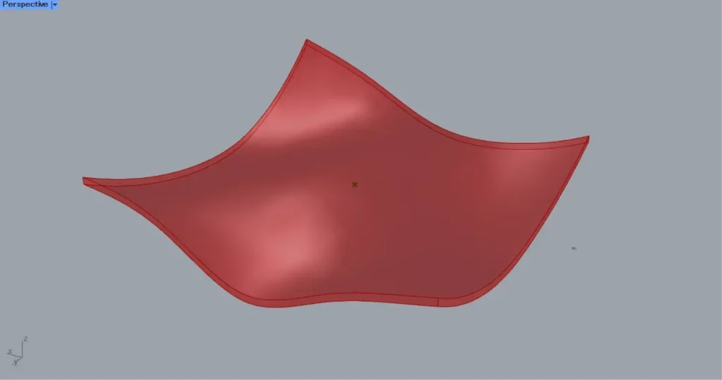
Then connect the Brep to a Volume.

Then you can get the center point of the model, as shown in the image above.

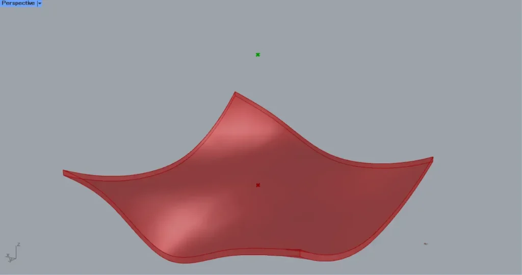
Then connect the numbers to be moved to au Unit Z.

This time, we connect 5000.

Then connect the Unit Z to a Move(T).

In addition, connect the Volume(C) to the Move(G).

Then the point moved directly upward, as shown in the image above.

Then connect the Move(G) to a XY Plane.

Then a plane is created at the location of the moved point, made of X and Y directions.

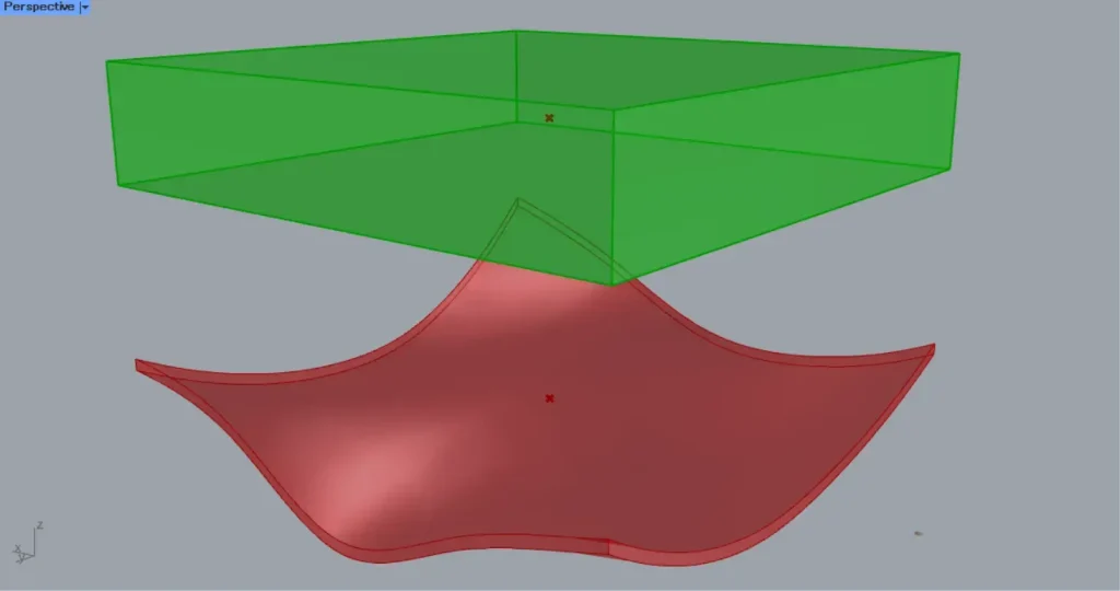
Then connect the XY Plane to a Center Box(B).

Furthermore, connect the 1/2 numbers on each side to X, Y, and Z.

This time, we connect 5000 to X and Y and 1000 to Z.

This creates a 10000 x 10000 x 2000 box centered on the point, as shown in the image above.

Then connect the Center Box to a Populate 3D(R).

In addition, connect the number of points to be created to the Populate 3D(N).

This time, 2000 are connected.

Then 2000 dots are created in the box, as shown in the image above.

Set up the model so that points can collide with the model

Next, we will set up the model so that points can collide with the model.

Connect the Populate 3D to a SolidpointCollide(Points).

In addition, connect the Brep to the SolidpointCollide(Solid).

Furthermore, connect False to the SolidpointCollide(In).

In this case, we use Boolean Toggle.

This causes collision detection to occur outside of the model.

In addition, we connect True to the SolidpointCollide(Uni).

This ensures that the model is not affected by collisions.

These settings in the SolidpointCollide causes points and models to collide.

Then connect the Populate 3D to a Load(P).

In addition, connect an Unit Z to a Negative.

This allows us to get a vector directly downwards with Negative, where the direction is multiplied by a minus and backwards.

Then connect the Negative to the Load(FV).

This apply a load directly down at each point.

Then connect the Populate 3D to a SphereCollide(Points).

Furthermore, connect the radius values to the SphereCollide(R).

This time, we connect the 50.

This makes the points collide, with each point having a radius of 50.

Then prepare a Floor.

This causes the points to stop at a height of 0.

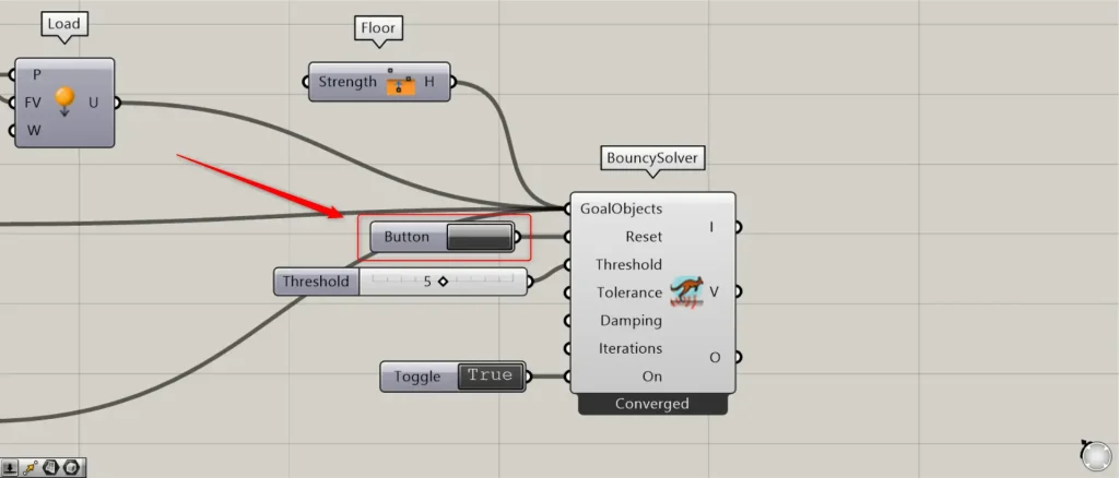
Then connect the SolidpointCollide, the Load, the SphereCollide and the Floor to a BouncySolver (GoalObjects).

In addition, connect a Button to the BouncySolver(Reset).

This allows you to run the analysis by pressing a button.

Furthermore, connect a threshold value(the value of how much it stops moving, at which point the analysis ends) to the BouncySolver(Threshold).

In this case, we are connecting 5.

If you do not set this value, the analysis will not finish or will be very long.

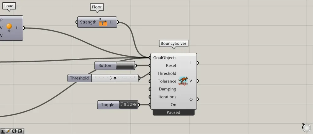
In addition, connect True or False to the BouncySolver(On).

If True, the analysis is ready to run.

If false, the analysis cannot be performed.

Initially, we set the value to False.

Run the analysis

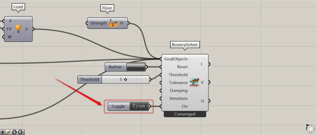
Set the state of the BouncySolver(On) to True.

Then press the Button.

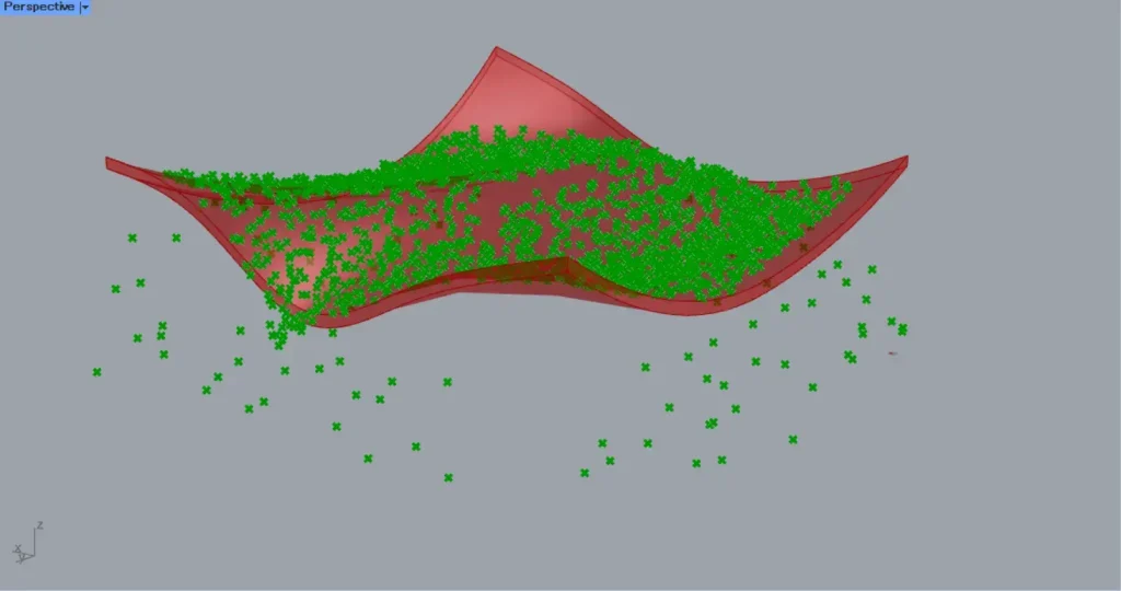
Then, as in the image above, points fall from directly above and analysis begins.

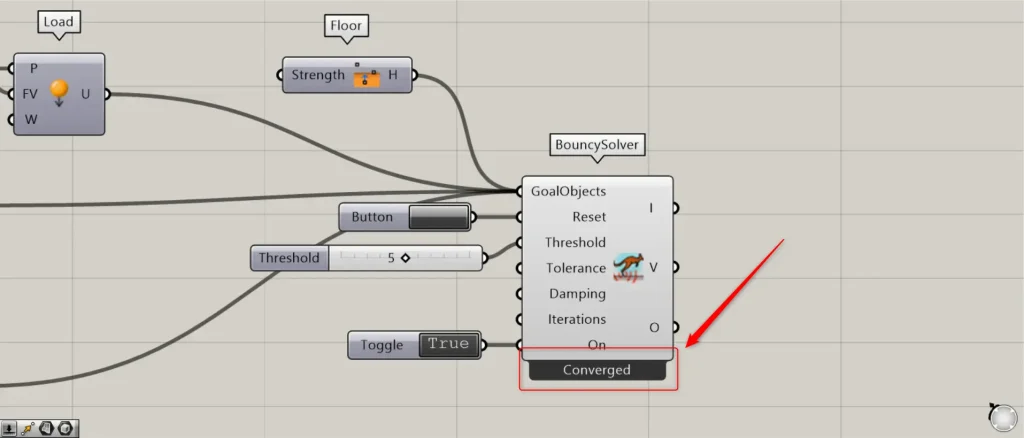
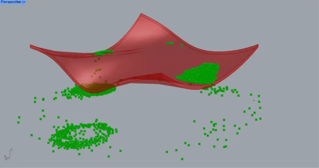
When the analysis is complete, Converged is displayed.

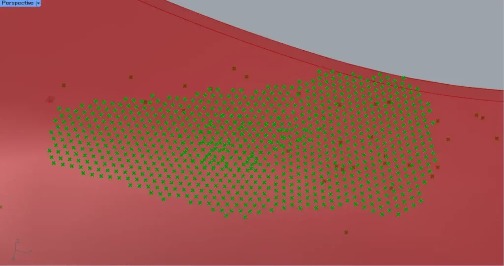
The radius is specified by the SphereCollide, so you can see that there is spacing between the points.

This completes the process.

That’s all for this issue.